2023-3-26 arXiv roundup: Unit scaling, Origins of power laws, Removing text watermarks
This newsletter made possible by MosaicML.
Unit Scaling: Out-of-the-Box Low-Precision Training
They make all the weights, activations, and gradients have unit variance through simple math. Unlike initialization schemes that try to get one of these (usually activations) to have unit variance, they get all three by:
Multiplying in a constant for each op
Letting the gradients be “wrong” by a fixed constant factor. So you’d need to update your learning rate and weight decay when using their method.
The basic observation here is that floating point causes the least quantization error when your values are near 1. So by giving all tensors an elementwise variance of approximately 1, you ensure that you have plenty of precision even when using few bits.
Of course, the challenge here is that if you multiply two matrices together with unit-variance elements, the result has larger variance. For an NxN matrix product with iid elements, the output elements will have a variance of N.
To fix this, we need an op-specific scale factor. E.g., for our NxN matrix product, we divide the output by sqrt(N) and we’re good. This is mathematically equivalent to just scaling down one of the matrices by 1/sqrt(N) but numerically much better. It’s better because a) our optimizer updates deal with unit-variance weights and b) we only see values far from 1 in our fp32 accumulators.
This need for a scale factor extends beyond matrix products, but you can easily derive the scales for other common ops. Note that there can be separate scale factors for forward (α), grad wrt input (β_X), and grad wrt weight (β_W) since they reduce along different axes.
One subtlety here is that you kinda get screwed by skip connections. If you add two iid matrices with a variance of 1, the sum will have a variance of 2. So you have to instead perform a “weighted” sum where you scale down the inputs.
Equipped with this ability to make ops have unit-variance outputs given unit-variance inputs, we can initialize + transform our model to have unit variance basically everywhere.
The other subtlety here is that, whenever you have parallel branches, you have to scale the gradients for each one the same way. If you don’t, your gradient can be wrong since the two branches’ gradients won’t point in identical directions. You can formalize this constraint in terms of whether cutting an edge in the compute graph would split it into multiple connected components.
To ensure the scales are the same, they just use the geometric means of the “ideal” forward and backward scale factors for each op in a branch, which sacrifices the guarantee of unit variance but makes the gradient exactly correct (instead of just up to a constant factor).
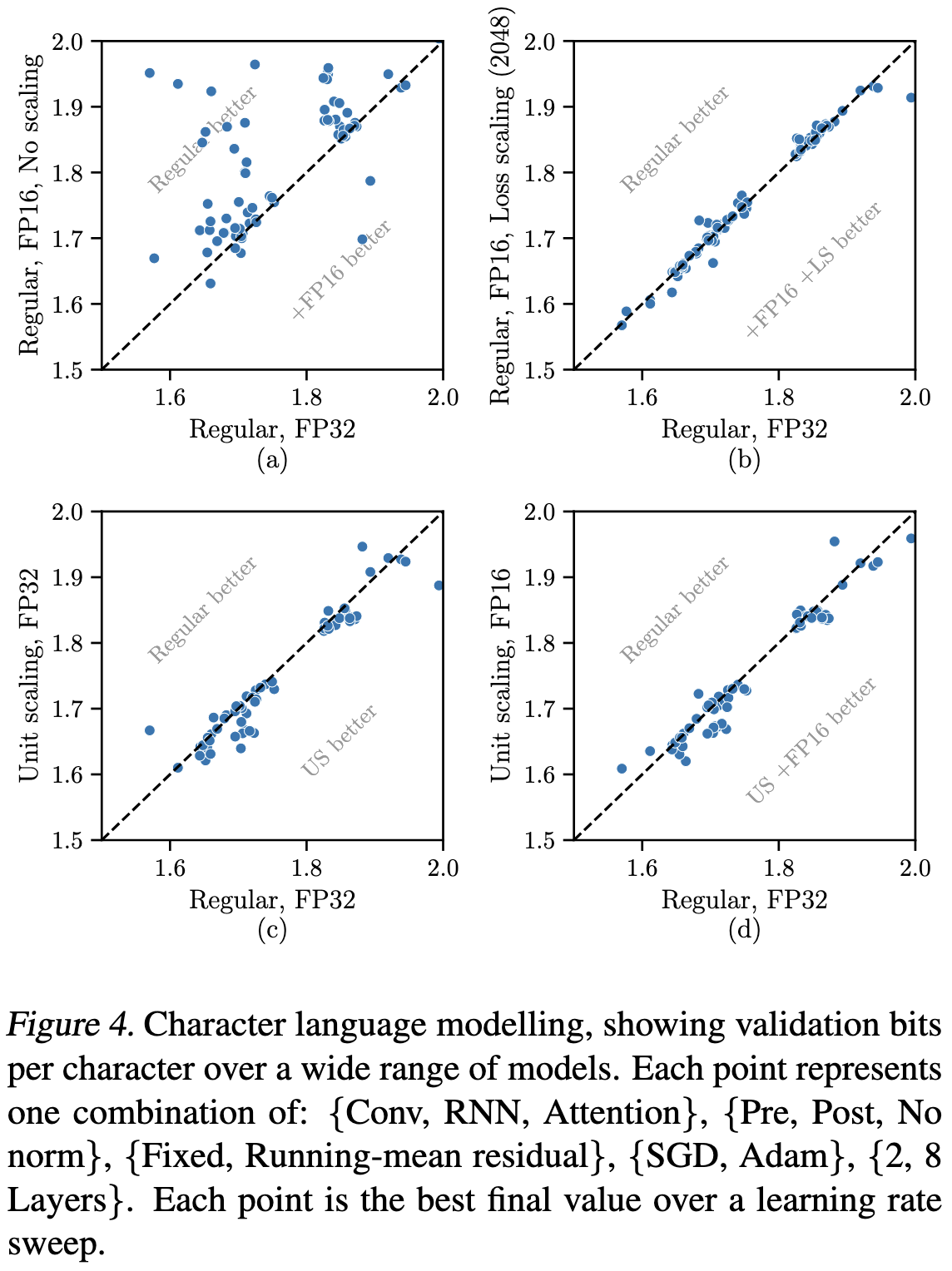
Empirically, their method tends to be almost indistinguishable from, or slightly better than, fp32 training (points in the lower right halves of the bottom two subplots). Each point here is a training run on a simple model using optimized hyperparameters.
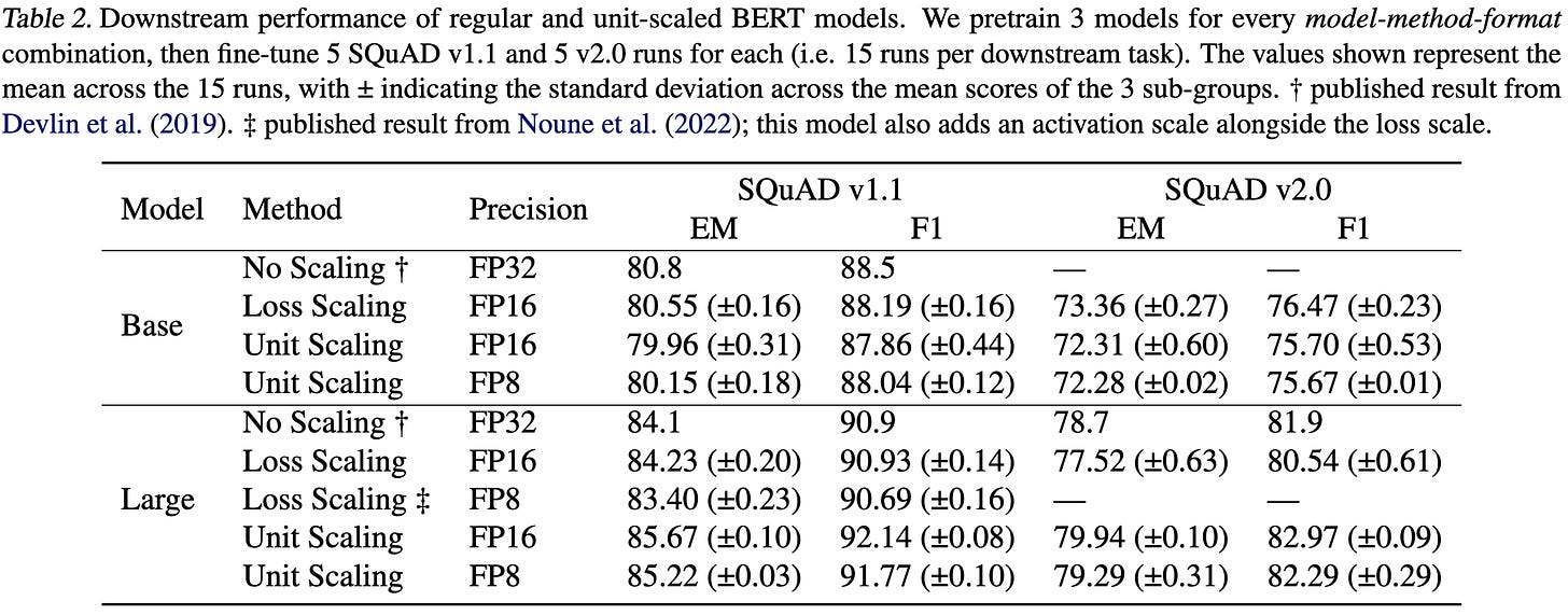
For BERT pretraining, they do about 1% worse than regular loss scaling for BERT-Base, but about 1% better for BERT-Large. Since they do better with fp8 than fp16 for BERT-Base, I suspect those numbers might just not have optimized hparams or something.
Overall I really like this. As an engineer, I just find it super elegant to go from first-principles analysis of ideal behavior to simple math that (roughly) guarantees this behavior. And the fact that they got fp8 training working at the same accuracy as fp16 is super cool. Plus it’s great news for NVIDIA’s Hopper cards, which have fp8 tensor cores.
What does it take to catch a Chinchilla? Verifying Rules on Large-Scale Neural Network Training via Compute Monitoring
Could you build a training system that allows companies to prove compliance to an external regulator? By compliance, we mean properties like how many FLOPs went into training, whether cybersecurity exploits were part of the training data, how much data you used, etc.
They argue that the answer is at least sort of yes under certain conditions. First, you need to be training on hardware with SGX-like functionality that records trusted snapshots of model weights throughout training. Second, you need some procedure for using logs of weights to check properties of the training that isn’t susceptible to spoofed logs. Third, you need various other pieces like stores of various hashes.
This isn’t practical yet since the second component—turning logs into guarantees about properties—is an open problem.
But it’s an interesting problem formulation that suggests fruitful research directions and made me think more concretely about AI safety.
CoLT5: Faster Long-Range Transformers with Conditional Computation
They split transformer blocks into a lightweight and a heavyweight branch, conceptually similar to Big-Little networks. Most of the tokens just go through the lightweight branch, while some go through the heavyweight branch.
The lightweight branch does local attention in a narrow window. The heavy branch selects a subset of queries and a subset of keys and does full attention between just those subsets.
The updated representation of a given token at the end of a block is just a weighted sum of the output from the light and heavy branches, plus a skip connection.
The weight associated with the heavy branch is a based on a 1d projection of the token’s current representation. This projection is also used to select the top k keys and queries to route through the heavyweight branch.
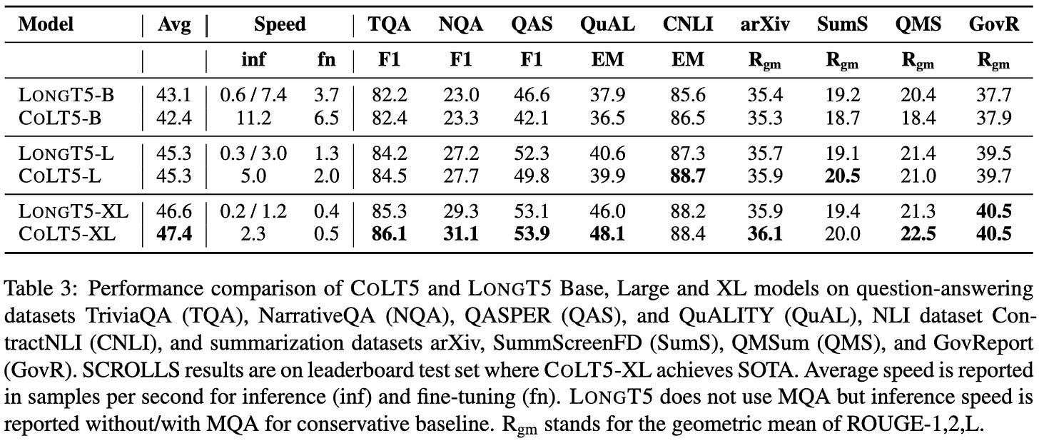
With the right hyperparameters for how many queries and keys to route to the heavy branch and how big your local attention window should be, you can get a much better speed vs quality than a relevant baseline.
One interesting consequence of their fast handling of long sequences is that you can trade off sequence length vs accuracy by adding more examples in the prompt.
Their ablation experiments suggest that most of their changes are meaningful. E.g., you need to select which tokens go through the heavy branch intelligently. Reassuringly, it doesn’t seem to matter much that they trained using the UL2 objective rather than PEGASUS (like their baseline).
Seemingly another win for conditional computation. Plus they reproduced benefits from multi-query attention.
Data-centric Artificial Intelligence: A Survey
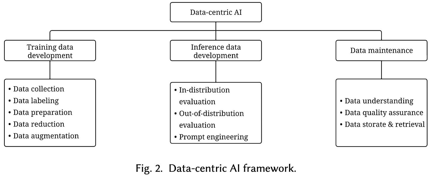
A big survey of methods for defining and improving your data pipeline.
This includes a ton of different aspects, most of which people have attempted to automate.
A good source of references if you’re trying to build a great data pipeline.
Can AI-Generated Text be Reliably Detected?
Not really.
From a practical perspective, you can just use another model to paraphrase the text and thus remove any watermarking.
Though this paraphrasing can degrade the text quality, at least if you do with a less advanced model than the one that generated the text. E.g., their results use a 1.3B parameter generator with a 222M parameter paraphraser.
If you have access to a particular detection API you want to fool (or a good proxy for it), you can also amplify your chances of fooling it dramatically by paraphrasing the text multiple times and taking the best one.
Worse, they prove a theorem stating that, as AI approaches exactly capturing the distribution of human-generated text, the best any text classifier could do approaches random chance.
Finally, they show that you can at least sort of learn the distributions of next tokens in watermarked text and use this to generate text that you know will get flagged as AI-generated.
This is kind of an argument for centralization of text generation capabilities; if you had to go through some API to get good AI text generation or paraphrasing, then presumably at least one provider would be able to watermark the final output. But of course, it’s kind of too late for that already, and centralization of power in extremely few hands comes with all sorts of other issues.
Stabilizing Transformer Training by Preventing Attention Entropy Collapse
It’s already known that self-attention tends to lose rank doubly-exponentially with depth, often leading to huge outlier features. This paper both further analyzes the problem and proposes a simple and effective solution.
As far as analysis, they prove a tight lower bound on the entropy of attention matrices and show that it tends to go down as the spectral norm of the attention logits increases.
To fix this problem, they propose to normalize all the weight matrices by their spectral norm (largest singular value) and scale them by a learned constant γ.
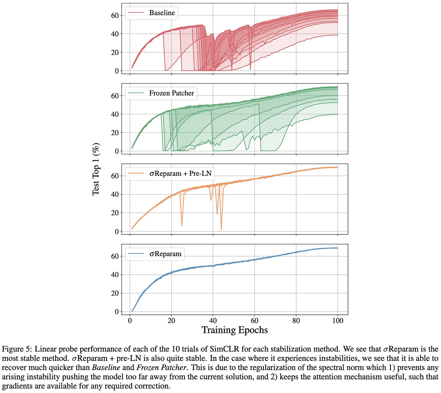
With this one change, they end up with much stabler training of ViTs on ImageNet,
self-supervised vision models,
and machine translation models.
The downside is that the method adds a fair amount of overhead. For one, you have to do fp32 power iteration to find the spectral norm for each matrix throughout training. Besides that, you need to compute a gradient with respect to each scale parameter, which is a going to be memory-bandwidth bound unless maybe you fuse it into the wgrad computation.
That said, this throughput hit could be worth it if it makes your training run actually converge.
The effectiveness of MAE pre-pretraining for billion-scale pretraining
Before you pretrain your vision model on image-caption pairs, you should pre-pretrain it with a masked autoencoding objective. This improves downstream accuracy across a variety of tasks.
The first result here is that, as you’d hope, this approach works better when you use larger models and datasets. In particular, using a 3 billion sample Instagram {image, hashtag} dataset works better than just ImageNet-1k.
Now, it’s not that surprising that throwing more compute at the training process gets you better results. The key question is whether you’re better off spending some of that compute on a separate masked pre-pretraining phase.
The answer is apparently yes. In the middle subplot, we see that you can do better for a fixed number of passes through the instagram dataset using a mix of both. In the right subplot, we see that you do better when holding training FLOPs constant (and FLOPs is actually a decent metric here since we’re holding the architecture ~constant).
What sticks out to me most here is the absence of power laws. They clearly varied model and dataset sizes, so the fact that they don’t report any suggests to me that they didn’t find them. Maybe power law scaling is more of a text modeling thing than a universal deep learning thing?
SIFT: Sparse Iso-FLOP Transformations for Maximizing Training Efficiency
(No, not the classic SIFT algorithm.)
They scale up the layers in a neural net while proportionally sparsifying them. This holds the FLOP count constant while greatly increasing the activation tensor sizes. They investigate making linears/convs wider, making parallel copies of layers and adding the results, factorizing, and mixing factorization with unstructured sparsity.
In terms of results, they have a nice ablation experiment showing how much better you can do with unstructured rather than N:M sparsity. The one caveat here is that ResNet-18 is an ImageNet architecture that downsamples aggressively at the start (in contrast to ResNet-20 and ResNet-56, which are for CIFAR). But I doubt this matters much here.
The big result is that making your layers wider + sparser works great in terms of accuracy vs FLOPs. This is consistent with previous findings, but it’s an unusually clear illustration of this principle.
The improvements for larger, sparse layers hold not just for CIFAR-100, but also for downstream detection and segmentation tasks.
In terms of wall time, the benefits are a bit less clear. They find that Neural Magic’s inference runtime realizes a 5.2x speedup at 90% sparsity and their CS-2 training chip realizes a 3.8x speedup at 90% sparsity. So they 10x the activations, 1x the FLOPs, 10/5.2 = 1.92x the inference latency, and 10/3.8 = 2.63x the training time.
Nice experimental results that suggest a path to consistently benefiting from sparsity if you can get enough wall-time speedup from it.
Also highlights that at least ResNets seem to have way too high a ratio of FLOPs and parameters to activations. Though it might not be that simple since structured matrix approaches also change this ratio and I’ve never seen a clear positive result with them.
The Quantization Model of Neural Scaling
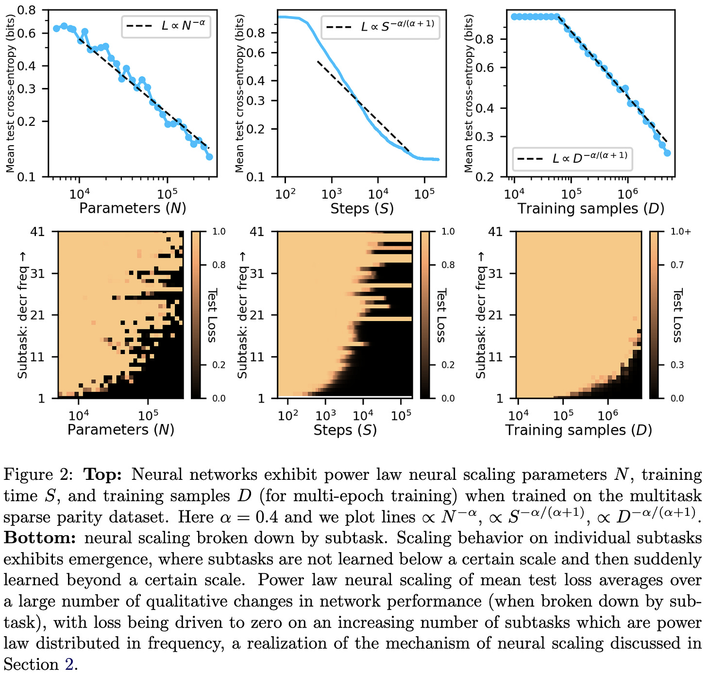
They suggest a mathematical model for why power law scaling emerges in language models.
Roughly, if
modeling text decomposes into discrete subtasks (“quanta”) like continuing numerical sequences or limiting line lengths,
the utility of learning different quanta follows a power law, and
the model learns higher-utility quanta first
you arrive at power law scaling.
Also, you kind of have to assume that learning a given quanta requires a fixed number of parameters and a fixed number of samples.
This model is consistent with some experimental results on a sparse parity learning task.
They also propose an algorithm for discovering quanta that seems to produce power-law quanta frequencies.
What I like about this is that it makes emergent behavior a natural part of scaling—it’s just new quanta being learned.
It’s also just really interesting. I derived a similar result a while ago that looks at learning tokens instead of learning quanta (since the former are known to follow a power law), but never came up with a story for how “learning a token” could actually be a thing. Talking about learning capabilities instead of tokens is much more consistent with experimental evidence.
The main shortcoming I see here is that we’re explaining power laws by just kind of assuming power laws. But it’s definitely interesting and the sort of work we need a lot more of. Even if they’re not 100% correct yet, we need unifying theories to test in order to make sense of deep learning.


