2023-5-7 arXiv roundup: Easy loss spike fix, LLongboi, H100s, stable diffusion for $50k
This newsletter made possible by MosaicML.
Thanks to Haoli Yin and Trevor Gale for the Twitter shoutouts this week!
Introducing MPT-7B: A New Standard for Open-Source, Commercially Usable LLMs
We released a family of 7 billion parameter models that work at least as well as other 7B models out there and often better.
They’re open source, available on Hugging Face, and hosted in Hugging Face spaces if you want to play with them.
One of the models—“MPT-7B-StoryWriter-65k”1—got a ton of attention for being able to handle context lengths of 65k+ tokens. This is enough to, e.g., feed in the entirety of The Great Gatsby and have it write an epilogue.
One of the coolest aspects of this release is that our training infra has reached a place where we could just set it and forget it. Like, here’s the logbook for our 9 day training run:
One hidden gem here is our fast eval harness; e.g., we added eval results for Together’s 7b model in 16 minutes.
It took a ridiculous amount of engineering and experimentation to reach this point, but we’re all super excited to be able to crank out high-quality models like this. Plus it’s been fun seeing all the community adoption + extensions that have come out in just a few days.
MosaicML Inference: Secure, Private, and Affordable Deployment for Large Models
If you want to query MPT-7B (or any other model) through an API, we now have a thing for that: MosaicML Inference.
Basically we kept helping customers train big models and they were like “can you help us serve it too?” So we were like “Okay, sure.”
The two offerings here are:
the “Starter” tier, where we host a fixed set of models you can query, and
the “Enterprise” tier, where we host any model you want in your own infra.
The Starter tier is basically the same deal as OpenAI’s APIs, but with open source models. Fun behind-the-scenes fact: this wasn’t on the roadmap initially, but we realized it was so easy to build by using our Enterprise offering ourselves that we decided to release it.
Benchmarking Large Language Models on NVIDIA H100 GPUs with CoreWeave (Part 1)
NVIDIA H100s are ~2.2x faster and 2x more expensive than H100s for 16-bit training, but 3x faster for fp8 training. And it looks like fp8 training “just works” for LLMs if you use NVIDIA’s TransformerEngine layers.
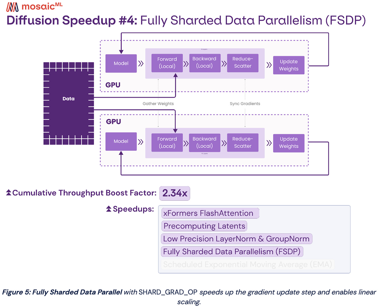
How We Trained Stable Diffusion for Less than $50k (Part 3)
We previously got Stable Diffusion training for $160k. Now we got it training even faster by:
using better attention kernels,
precomputing the outputs of the VAE and CLIP encoders,
using 16-bit norm operations instead of 32-bit,
configuring distributed training well,
and using an exponential moving average of the weights, but only at the end of training when it actually matters.
The details are kind of interesting, but the big picture is even more so; this is a 3x cost reduction in just a few months, which is a crazy rate of progress.
PyTorch FSDP: Experiences on Scaling Fully Sharded Data Parallel
The team behind PyTorch FSDP wrote a paper about it. We use FSDP at Mosaic for our LLMs and Diffusion Models, and have consistently gotten high utilization with it.
The basic idea with FSDP is to keep some combination of parameters, gradients, and optimizer states sharded, and then have each GPU allgather the full tensors when it needs them. So, e.g., you gather all the parameters for your FFN before using it in the forward (or backward) pass, and then free these materialized tensors as soon as you’re done.
There are a bunch of variants of this, and the way to think them about them is as different patterns of caching vs eviction. Here “caching” means materializing the full tensor in each GPU and “eviction” means freeing that tensor, retaining only this GPU’s shard of it.
If you cache the weights right before you need them in forward and backward and then immediately evict them, you have Zero-3.
Note that this never requires caching the full gradient or optimizer state tensors.
If you instead cache the weights in forward and don’t evict them until after the optimizer step, you get Zero-2.
If you also cache the gradients for each parameter and only evict them (via reduce-scatter) right before the optimizer step, you get Zero-1.
If you cache everything all the time and allreduce your gradients before the optimizer step, you have DDP.
There are two reasons that building something like FSDP is hard. First, you have a bunch of speed considerations. In particular, you never want to launch a communication operation on small tensors or imbalanced shards.
And when you do launch a communication operation, you want to make sure it runs in parallel with compute.
The second reason is that there are a ton of edge cases. How do you deal with initialization when your parameters can’t all fit in RAM at once? Or gradient clipping when your gradients are sharded? When the user asks for the shape of a sharded parameter, do you return the shape of the full tensor, or just the shard?2
So what does FSDP do? It enables several patterns of caching/eviction, but in general it:
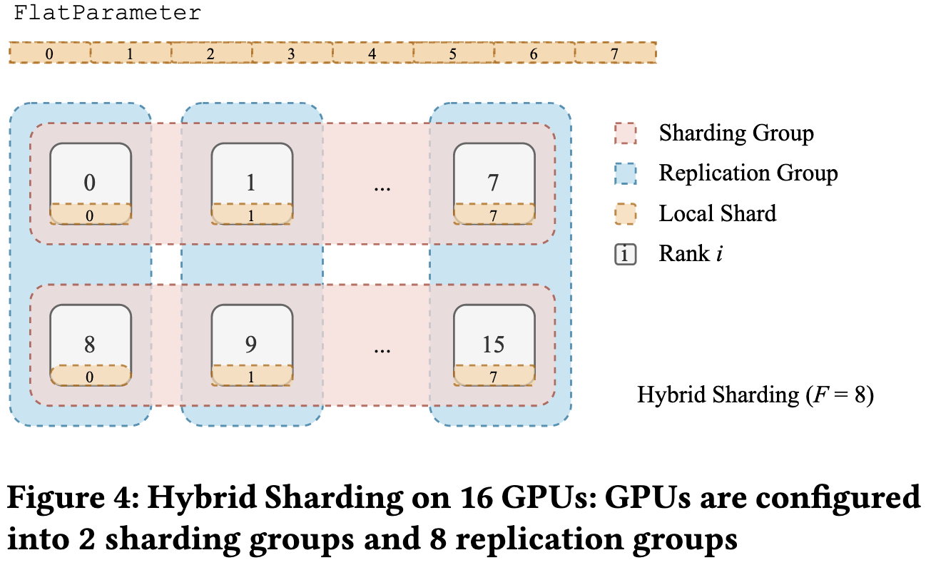
Coalesces a bunch of parameters from one or more modules into a single big “FlatParameter”. This helps improve communication throughput.
Prefetches the FlatParameters as needed in forward and backward.
It also allows you to do a mix of sharding and replication for each parameter tensor. Sharding requires more communication but uses less RAM, so this is a space vs communication tradeoff. The killer app for this is training across pods of dense interconnect in a datacenter with slow interconnect between the two pods; e.g., in public clouds, you’ll often hit a breakpoint at 512 GPUs.
As you might expect, these optimizations get them pretty good throughput across a variety of models with different hardware and batch sizes.
Here are the parts of this paper that stuck out to me—I would skip this if you’re not into thinking about the guts of distributed training.
They handle initialization not just by allowing use of the meta device, but by recording and replaying operations on the param tensors. At Mosaic, we always just pass in a callback to initialize tensors once they’re on the GPUs, so I didn’t know this was a thing. They mention this being necessary to support initializations with complex logic, but I’m not sure what use cases need this.
They had to prevent the prefetching from getting more than two FlatParameters ahead of the execution or they hit issues with the caching allocator. This rate limiting hurt throughput ~5% sometimes but prevented huge slowdowns on some workloads.
They do their communication in a separate CUDA stream that they manually manage and sync with and I’ve never understood why. Apparently it’s because “the ProcessGroupNCCL implementation has one internal NCCL stream per device.” But my cursory inspection of the code doesn’t suggest this, so maybe it’s a legacy thing (or my inspection was just too cursory)? Also NCCL manages a separate communication stream internally, so maybe the goal is to use the semi-supported ability to have multiple concurrent communication ops running in different streams? I guess this could help if you aren’t saturating your links with one collective op.
Instead of making their allgathers differentiable (to let autograd kick off the reduce-scatters automatically), they manually add post-backward hooks to the tensors and manage the reduce-scatters themselves. I guess this gives you more control, but I’m not sure what the benefit is.
Speed Is All You Need: On-Device Acceleration of Large Diffusion Models via GPU-Aware Optimizations
They introduce a bunch of optimizations to speed up large diffusion models.
These optimizations are mostly fused kernels + Winograd convolution.
Interestingly, they do a little bit better than FlashAttention on some hardware with an alternate fusion scheme.
Always nice to see measured speedups on real hardware.
Efficient Training of Deep Equilibrium Models
Deep Equilibrium Models approximate repeating a block of the network an infinite number of times. This gets you (hopefully) more expressive power per parameter and almost no increase in memory compared to just applying the block once, but has two downsides.
The first downside is that it’s reportedly hard to get these models to work reliably—in particular, you need the output activations of the block to converge to some fixed point, which, in general, they might not.
The second issue is that you have to solve for the fixed point you would reach if you applied the block infinitely many times, as well as the resulting gradients. You can do this more efficiently than naively unrolling it many times, but it’s still kind of slow.
This paper helps with the second issue. Their approach is to reuse the approximate Jacobians you use when solving for the activations in the forward pass to compute the gradients in the backward pass.
This approach seems to do better than previous methods on CIFAR-10.
The Disharmony Between BN and ReLU Causes Gradient Explosion, but is Offset by the Correlation Between Activations
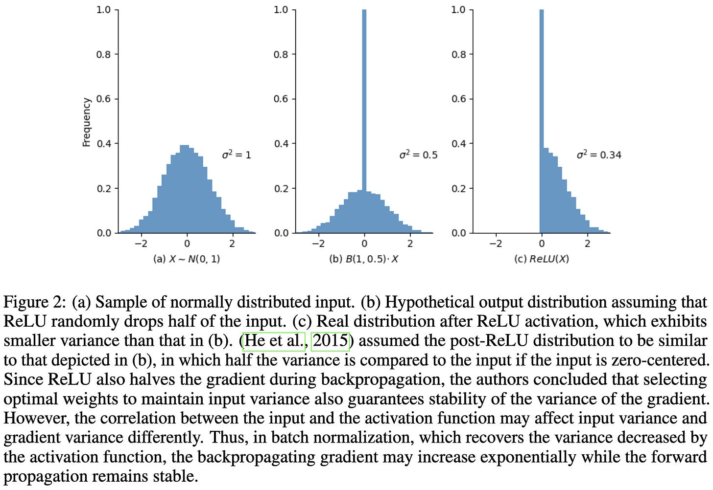
Let’s start with an observation: ReLU and other nonlinearities produce outputs with lower variance than their inputs.
A consequence of this is that batch normalization layers scale up the activations. And this also means that they scale up gradients in the backwards pass. Since ReLU and other nonlinearities might not reduce gradient variance by the same amount in the backward pass as they do in forward, this can cause gradients to explode as you get earlier and earlier in the network.
Nonlinearities can reduce the variance less if a lot of inputs are in the high-slope regime of the activation function, and reduce it more of a lot of inputs are zeroed out or in the low-slope regime of the activation function.
They describe conditions under which we can avoid these issues:
Based on these observations, they propose an optimization algorithm that should avoid exploding gradients.
They don’t show experimentally that this approach fixes the gradient norms, but it does seem to do about as well as other optimizers for ResNet-50 on ImageNet even without learning rate warmup.
It’s well known that batch norm can cause exploding gradients, but this paper has some nice figures and math to help further our understanding of this issue.
A Cookbook of Self-Supervised Learning
A survey of SSL methods with an emphasis on helping you get started using them. Curates results from various papers and has mini-tutorials on key ideas.
Patch Diffusion: Faster and More Data-Efficient Training of Diffusion Models
They do diffusion on random patches (augmented with coordinates) instead of full-sized images. The coordinates are (x, y) positions expressed as a 2-tuple of values in [-1, 1], added as two extra channels.
More precisely, they randomly choose between training on full-sized images, half-resolution patches, and 1/4 resolution patches in each batch.
For 64x64 images, changing the fraction of full-resolution images trades off quality vs training time.
Their overall method can reduce training time ~2x while often preserving generation quality.
Seems promising, especially given how well similar techniques work for image classification.
What Causes Exceptions in Machine Learning Applications? Mining Machine Learning-Related Stack Traces on Stack Overflow
A bunch of different stuff. Python syntax errors are the #1 culprit.
Noise Is Not the Main Factor Behind the Gap Between SGD and Adam on Transformers, but Sign Descent Might Be
People have suggested that Adam might outperform SGD for transformers on text data because of the long tails in the stochastic error. By “stochastic error,” we mean the difference between the true gradient direction and the gradient direction derived from one minibatch.
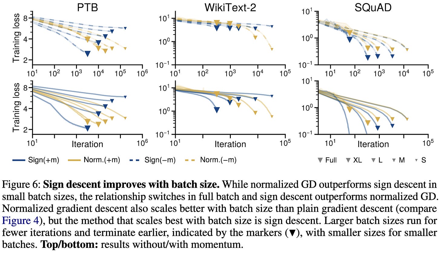
But this appears to not be the explanation, in that they still observe a gap when doing full batch training.
Interestingly, the gap tends to widen as the batch size increases (holding iteration count constant, but not necessarily samples).
What might be happening is that Adam is better at exploiting low-noise gradients than SGD is.
A related question is what aspects of Adam make it work better. To test this, they rerun the above experiments with simplified alternatives (sign descend and normalized gradient descent).
Sign descent tends to do better than normalized gradient descent at large batch sizes but worse at small batch sizes.
With a large enough batch size, sign descent gives you almost all of the benefit of Adam. This is consistent with findings (including ours) that LION works at least as well as Adam for text transformers.
But it’s still not clear why this would only apply to text + transformers and not images + CNNs. Or why sign descent should work so well.
Nice to see all these controlled comparisons and simple baselines—we need a lot of more of this as a field, including to answer the above open questions.
DataComp: In search of the next generation of multimodal datasets
They have a standardized {pool of samples, training script, eval harness}, and the challenge is to curate/clean the dataset as well as possible.
They also contribute a big, filtered dataset of image-text pairs from Common Crawl.
Using a 1B subset of this dataset often yields better downstream results than LAION-2B.
They also perform various experiments to understand dataset scaling.
For constant data quality, more is more. But when you start filtering well, there’s an optimal point that trades off quality vs quantity. Also, the gains from filtering can be huge.
Encouragingly, filtering strategies that work well at smaller scales tend to work well at larger scales too.
Seems really valuable; hopefully this will help the field do less model science and more data science (as is common in industry).
We're Afraid Language Models Aren't Modeling Ambiguity
They made a text dataset with different kinds of ambiguity and looked at how well various models did on it.
The data collection pipeline starts with sentences generated by InstructGPT but gets gold standard labels from linguists.
Turns out LLMs are still not great at dealing with ambiguous sentences.
I really like how various specialized datasets are popping up to help us identify failure cases. We might reach a point where we can reliably unit test our text models and be confident about their efficacy on various tasks.
Cuttlefish: Low-rank Model Training without All The Tuning
They managed to get a training speed vs accuracy improvement for [Wide]ResNet-50 on ImageNet by factorizing the model part of the way through training.
They don’t bother factorizing a given layer unless it makes it faster in terms of wall time.
You have to set some hparams for, e.g., where to cut off small singular values, but given those hparams the algorithm automatically selects what rank to use for each layer.
Impressive that they actually got a time vs accuracy improvement with factorization. Usually factorization papers just get {FLOPs, param count} vs accuracy improvements at the expense of memory bandwidth + arithmetic intensity.
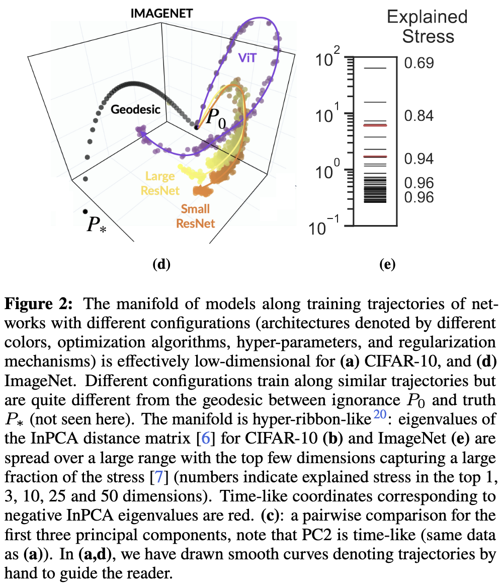
The Training Process of Many Deep Networks Explores the Same Low-Dimensional Manifold
The way they measure it is a little complicated, but basically if you look at the patterns of predictions over time embedded in a low-dimensional space, you see similar trajectories for different architectures. This holds even across different hparams and kind of even across model size. The trajectories also live in low-dimensional manifolds within the embedding space.
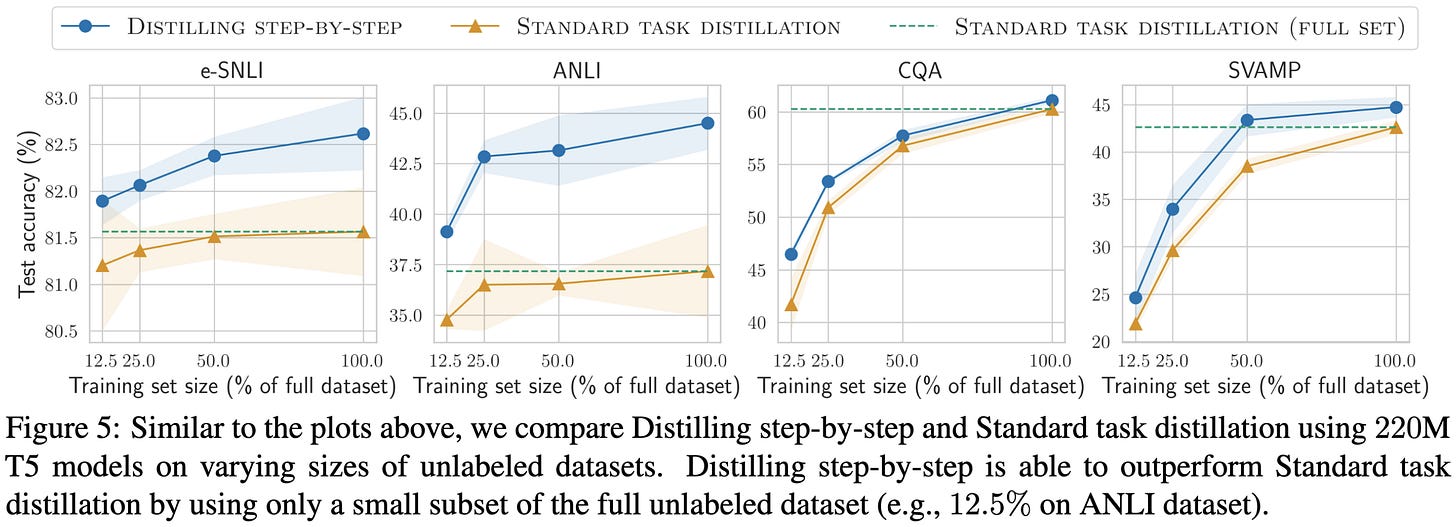
Distilling Step-by-Step! Outperforming Larger Language Models with Less Training Data and Smaller Model Sizes
They generate way more training data for a given downstream task by having a pretrained model generate rationales and (if needed) labels for a given input.
This extra supervision gets them huge accuracy lifts, to the point that they can get away with much smaller models and/or less downstream data.
To get rationales out of their pretrained LLM, they use chain-of-thought prompting with around 10 in-context examples that include rationales.
To use this extra data, they train the smaller downstream model to either predict the label or the rationale, with a special task token at the front to tell it which one to do.
Adding the extra training to predict rationales works way better than just training on the original downstream data. You can use these accuracy gains to train smaller models on less data while preserving accuracy.
Their method also works better than “standard task distillation”, by which we mean treating the teacher model’s outputs as labels.
Seems like a large, practical improvement. It’s also interesting that it does better than more conventional distillation.
Makes me curious how much of this is from rationales being especially high quality supervision vs rationales just being more supervision (longer strings) vs rationales just making us crank up our total training compute.
Also cool to see controlled comparisons of big generalist models to small specialist models, and just how much smaller the latter can be at a given accuracy. This is a) super important if you care about inference cost and b) part of why one model is unlikely to rule them all.
Dynamic Sparse Training with Structured Sparsity
They do N:M sparsity with a fixed number of nonzero weights per neuron, weight un-pruning based on gradient magnitudes, and occasional removal of entire neurons. The result that stood out to me here is that they got 75% structured sparsity with 1% accuracy loss; this probably isn’t worth it in terms of speed vs accuracy, but it suggests that you might be able to get almost no accuracy loss at 50% sparsity (which is the amount that recent NVIDIA GPUs can exploit, and therefore a possible speed vs accuracy win).
Cheaply Evaluating Inference Efficiency Metrics for Autoregressive Transformer APIs
They devise a procedure to estimate how efficient the inference is for different black-box text generation APIs. They also compare this to the capabilities these APIs offer.
First, they observe that an autoregressive text model’s inference time is an affine function whose bias is the prompt encoding time and whose slope is the per-token generation time.
Next, they measure the empirical latency of different APIs. There’s additive noise here, so taking the minimum gets you a good estimate.
There’s also some subtlety you can model associated with how many queries you run in parallel. Apparently you can single-handedly slow some of these APIs down if you fire off a bunch of queries in a small enough window.
The last measurement is how long the models take to run on standardized hardware with a standardized software stack. You can measure this because the models are simple and their hparams are public.
If you compare the API latencies to the latencies in a standardized setup, you get a view of how well different API providers have optimized (or at least parallelized) their inference. OpenAI APIs seem to be the most optimized, followed by AI21.
It’s much less clear who’s doing the best if you control for accuracy though.
Also, they have a table of how long different public APIs take to run as a function of prompt and output length. You might care about this if you’re sensitive to latency or want to know how well your own inference stack is doing.
ZipIt! Merging Models from Different Tasks without Training
They propose an algorithm to combine two models with the same architecture and input space but potentially different output spaces.
This is cool because existing work on combining models focuses on the case of shared output spaces.
It’s also interesting because it doesn’t require the combined model to be a convex combination of the input models after permutation.
They achieve this by, conceptually:
Concatenating the weights for the two models to form a combined model that’s twice as wide.
Learning matrices M and U for each linear op that project this wider representation down to the original width while still capturing most of the variance.
Fusing M into this layer and U into the next layer; this way, they never have to materialize a widened layer and preserve the original architecture.
Crucially, this formulation allows merging features within each model, not just across models. This apparently makes the merging work way better.
The tricky part here is dealing with nonlinear operations. To do this, they merge in elementwise layers as needed.
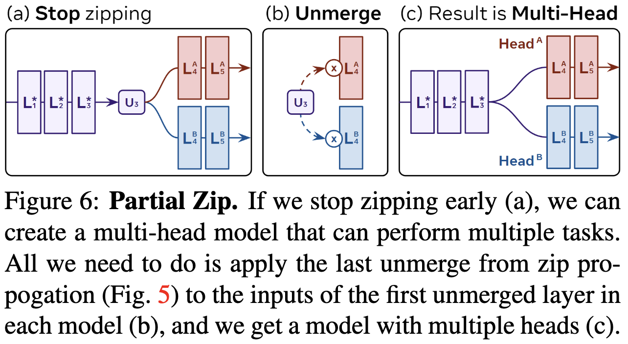
They also note that you don’t have to merge the models completely. If you only merge a prefix of the models, the unmerged suffixes can be task-specific heads.
This approach works better than other model merging methods when the output spaces differ. It’s not amazing in absolute terms though; merging two models that are each ~36% accurate on half the data would yield ~18% accuracy if you just chose between the two at random, while merging the models obtains 8.6% if you zip all the layers.
But what’s really happening here is that there’s an accuracy vs {time, space} tradeoff you can tune by adjusting how large a prefix of the model to zip (with the suffixes being separate task heads). If you only zip a small prefix, you don’t get much accuracy loss.
This probably won’t get you the same model quality as any sort of multitask learning scheme, but the results are still super impressive this they’re all evaluated with no training after the merge. Usually messing with a trained model at all-especially in the early layers—torpedos your accuracy, so this is super impressive.
It also makes me wonder how much of what we attribute to [permuted] linear mode connectivity actually has to do with the structure of the loss landscape—as opposed to just being a result of low-rank matrices in high dimensions. Like, maybe you can just always stitch together piles of linear algebra without even thinking about the loss landscape or its modes.
If so, that’s great news for efforts to make models composable.
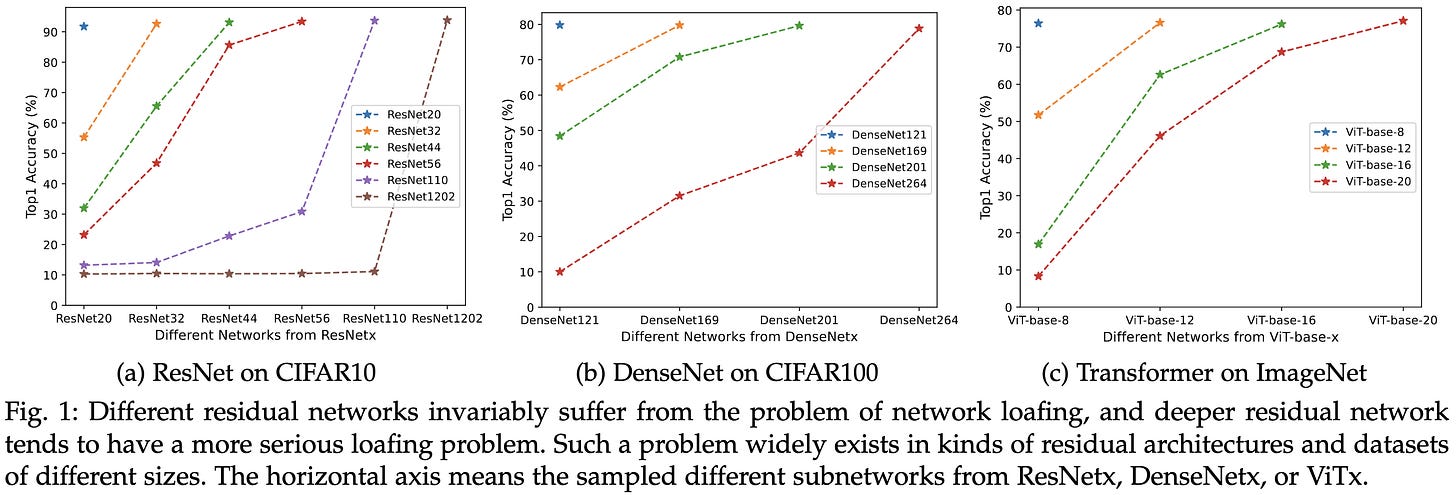
Stimulative Training++: Go Beyond The Performance Limits of Residual Networks
Here’s an observation: the first 50 layers of a ResNet-101 are way worse at predicting the label than a ResNet-50.
This suggests that the earlier layers are underutilized, which they term “loafing”. They propose to fix this by training random subnetworks. They penalize differences in predictions between the subnetwork and full network.
Unlike stochastic depth, they only sample random prefixes of the network to use as subnetworks.
This technique can lift ImageNet accuracy by several percentage points.
It also seems to help for a variety of other tasks when using ResNet-50 as a backbone.
Mostly I want to know how this compares to conventional training for the same amount of time, since there’s extra overhead to compute outputs from both the subnetwork and full network. But it looks promising as a self-distillation strategy you can apply in a single training run.
I’m also reading this as evidence that stability/optimization is not at all a solved problem and early layers are likely undertrained in many cases.
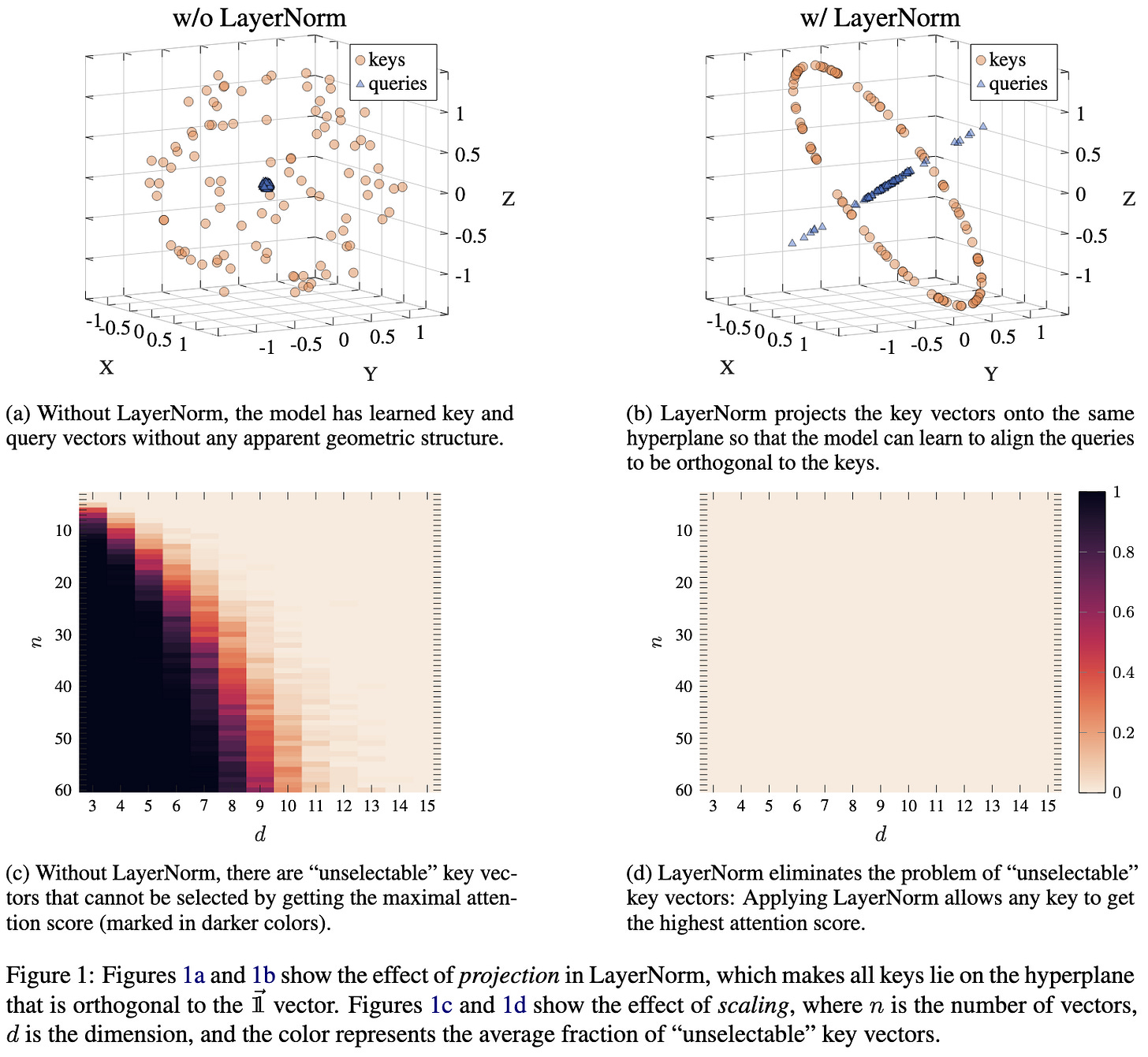
On the Expressivity Role of LayerNorm in Transformers' Attention
Adding layernorm before attention has two nice properties regarding attention’s expressivity:
It makes it so that queries can weight all coordinates equally to attend equally to all keys. This is helpful for stuff like computing a majority vote.
It makes it so that no keys are within the convex hull of the other keys. I’m not sure this happens in high-dimensional spaces, but in theory you could have a key vector whose magnitude is so small that even a query that perfectly aligned with it would have higher inner product with some other key.
Always nice to get a dose of insight about the semantics of different operators.
Stable and low-precision training for large-scale vision-language models
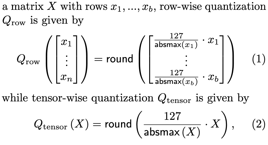
They matched 16-bit accuracy with part of the network quantized to int8 during training. The basic approach is to quantize the inputs to all the matrix multiplies using scale factors computed just-in-time to include the full range of observed values in each input. The scale factors can be unique to each row or shared for a whole matrix. After the matmul, they convert back to higher precision.
The method comes in three variants: SwitchBack, SwitchBackM and SwitchBackQ. The former does just-in-time tensor-level quantization. SwitchBackM adds quantization of gradients for the backwards pass, trading space for time overhead. SwitchBackQ is like SwitchBack but uses row-wise quantization.
The part that sticks out here is that they do int8 for the forward and input gradient computations, but need 16-bit for the weight gradient computation. This might be because their CLIP models have a huge token count per batch relative to the number of features, so that the wgrad sums over many more elements.
Vanilla SwitchBack makes linear layers run up to 35% faster.
It’s not the full ~2x speedup you’d get from pure int8 ops because of the quantization + dequantization overhead and the 16-bit wgrads. There also seems to be a lot of other (framework?) overhead, as evidenced by the gap in the two lines below on the right; here, calling F.linear is way faster than writing your own autograd function wrapping a matmul.
In terms of accuracy, SwitchBack gets you training curves that are nearly identical to those of bf16 training.
That’s part 1 of the paper. They then have a bunch of analysis of training [in]stability in CLIP.
First, they identify a few factors that make loss spikes more likely. These include larger model size,
larger batch size,
and larger learning rate.
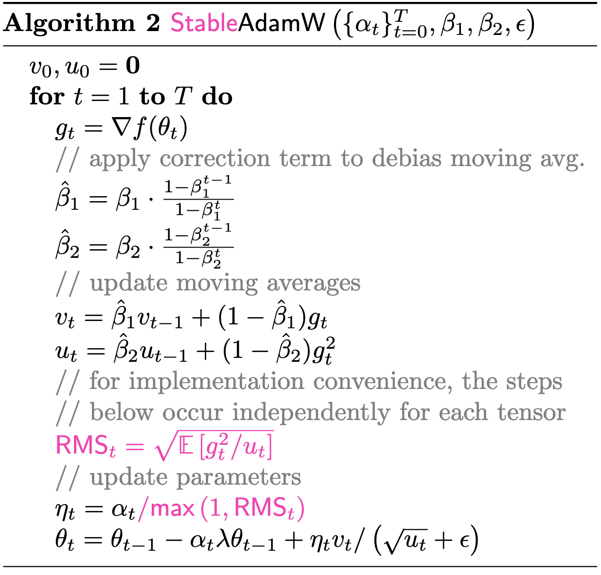
You can mitigate the spikes in all cases by just reducing Adam’s β2 hparam. This ensures that sudden, large gradients expand both the numerator and denominator. I’m pretty sure the largest update possible is (1-β1)/(1-β2 + ε), which happens in the case that you have an infinite history of zero gradients and then get a nonzero one.
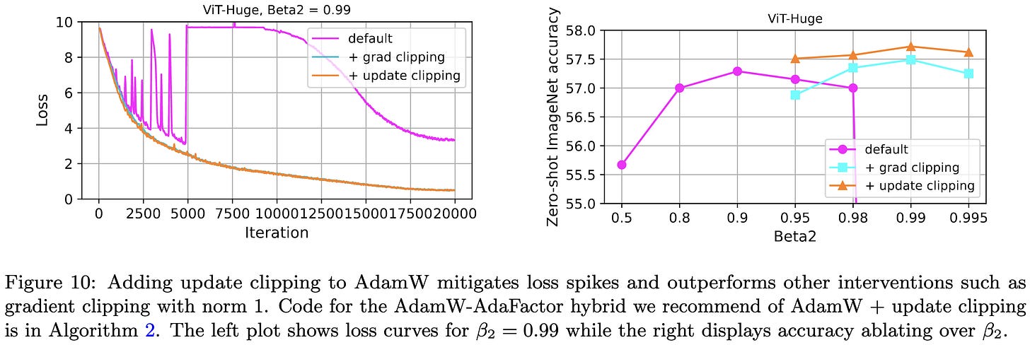
Based on this observed β2 sensitivity, they propose a modified AdamW that limits the maximum update size in a manner similar to AdaFactor. If the ratio of squared gradient to denominator is too large across a given parameter tensor, they clip the update.
They find that you get the highest accuracy with ViT-Huge on ImageNet by clipping the Adam updates, rather than clipping the gradients or doing nothing. This is interesting IMO since it’s a clean demonstration of instability causing not just outright divergence, but subtle degradation of the model. This suggests that improved stability could improve models.
In other news, to get simulated fp8 training working, they had to add learnable scales to each residual branch before the skip connection, and initialize these scales to zero. Without this, you end up with the residual stream growing too much with depth.
Finally, they confirm that spikes in loss often coincide with spikes in gradient and/or activation magnitude.
This paper makes me feel like we’re all a bunch of idiots, in a good way. Like, basic algebra shows that the maximum Adam update is proportional to 1/(1-β2 + ε)—and just sweeping β2 was apparently enough to confirm that it does, in fact, have a huge effect on whether we get loss spikes. This was kinda sorta known (c.f., AdaFactor, A Theory On Adam Instability, etc.), but it’s certainly not on most people’s minds and I've never seen such a clean demonstration of it before.
On the other hand, the fact that something so simple eluded us for so long is encouraging—it suggests that there’s still room to improve common practices and still reason to examine training from first principles.
I have a document with like 60 of these edge cases. Distributed systems are hard.






















this is great content!
How does the merge operation from the branch-train-merge differ from that of the Zip-it paper? It seems that combining the ideas of branch and train for domain experts along with the zipping operation removes the explicit routing needed?