2022-7-10 arXiv roundup: DeepSpeed inference, Simpler detection backbones, Spatial sparsification
This post made possible by MosaicML. If you like it, consider forwarding it to a friend!
DeepSpeed Inference: Enabling Efficient Inference of Transformer Models at Unprecedented Scale
DeepSpeed released an inference engine for huge models that lets you parallelize them across up to 256 GPUs.
There are a lot of optimizations to make this possible, spanning the whole compute stack. At the lowest level, they wrote a bunch of optimized CUDA kernels for small-batch inference. They also use PyTorch’s CUDA graph support to reduce per-op overhead.
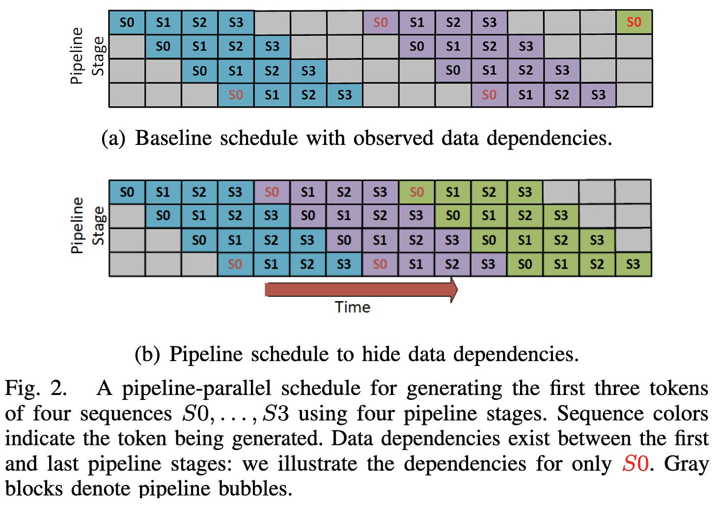
They do model parallelism within a node and pipeline parallelism across nodes. Note that pipeline parallelism is hard in the presence of serial decoding because of the data dependencies, plus the different treatment of prompt vs generated tokens. They end up using different microbatch sizes for the prompt processing vs serial generation.
They also interleave the token generation for different sequences to hide the data dependencies and avoid pipeline stalls. I.e., the outer loop is over output token position and the inner loop is over the batch.
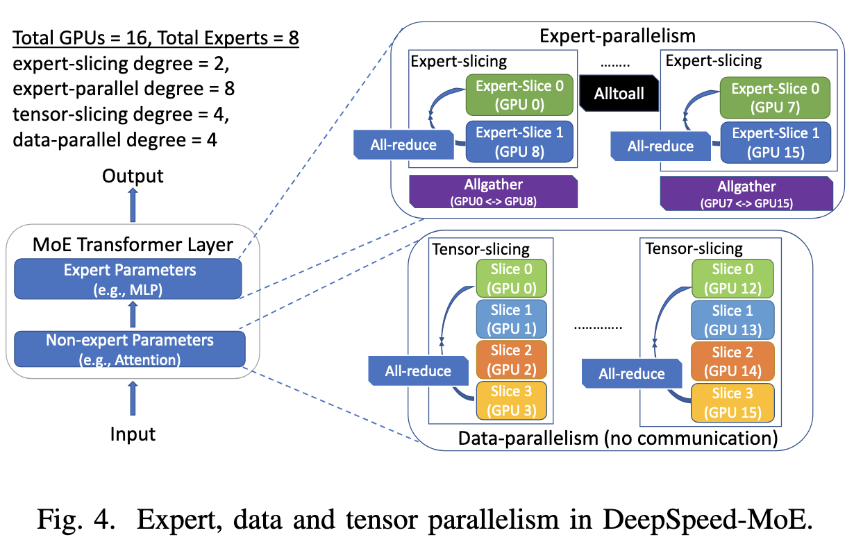
They also incorporate DeepSpeed-MoE, which is a whole separate feat of engineering we’ve covered previously.
One unorthodox design choice is that they keep the model weights in RAM or on NVME drives and stream them in as needed. This works because 1) they’re focused on models with huge individual layers; e.g., they point out that one GPT3-175B layer requires ~7 TFLOPs per input, and 2) they’re not necessarily assuming a batch size of 1.
There are a couple optimizations to speed up the weight streaming, including 1) prefetching upcoming layers to hide latency and 2) sharding weights across GPUs in a node during streaming, and then syncing between GPUs over NVLINK. If you aren’t a weirdo who’s memorized these numbers, PCI-E Gen4 is about 64GB/s, while NVLINK on A100s is about 600GB/s, so this two-stage process makes sense.
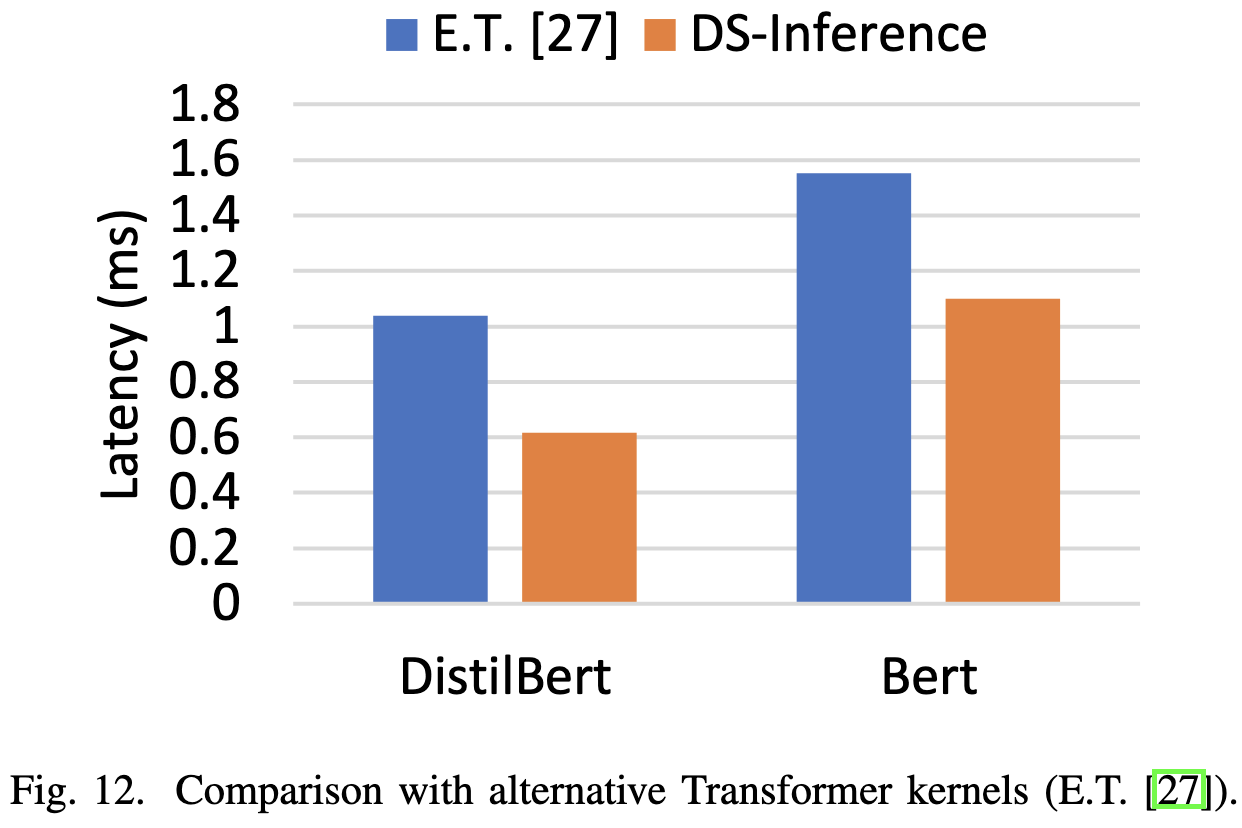
All these optimizations let them generate tokens much faster than previous work.
The improvements are especially pronounced for large-scale expert-parallel MoE models. Note that they managed to parallelize this across 256 GPUs, which is more than I’ve ever seen someone do inference on before.
This must have been a huge pain to build, but seems like exactly the right tool for the job. We’ve gotten away with single-GPU or single-CPU inference for a long time as a field, but systems like this are slowly going to become mandatory as huge models become more common.
Vector Quantisation for Robust Segmentation
They add vector quantization with 1024 centroids in the bottleneck layer of their U-Net. They use the straight-through estimator to generate gradients through the (non-differentiable) quantization operation.
They find that this simple intervention often improves accuracy and robustness. In fact, one can even prove certain robustness properties with respect to perturbations in the latent space.
Dynamic Spatial Sparsification for Efficient Vision Transformers and Convolutional Neural Networks
They route some fraction of the tokens in each image to the original FFN block and the rest to a simple linear projection. The fraction assigned to the slow path (full FFN block) diminishes deeper into the network.
Uses Gumbel-softmax sampling to get a gradient through the hard assignment operation. There’s also some subtlety in selecting a fixed number of tokens to keep for all samples in a batch; they handle this by keeping all the tokens but applying sparse masks to the attention matrices—this means they save no work in the attention computation. Although this shouldn’t matter too much since the FFNs are more likely to be the bottleneck unless you have unusually long sequences.
They assume that they start off with a pretrained vision transformer and distill the sparsified version from the original’s predictions. The distillation loss tells it to mimic the original models’ outputs for each token.
They also add cross-entropy losses for mimicking the teacher’s label distribution and the true label distribution, as well as an MSE loss for the fraction of nonzeros in the masks in each stage of the pruning.
Seems to improve FLOPs vs accuracy tradeoff significantly vs Swin Transformers—more so than most other vision transformer proposals.
There are quite a few degrees of freedom here and it seems like it was hard to get this to work, but I definitely buy the basic idea—doing different amounts of computation for different parts of the image makes a lot of sense. People have been proposing methods of doing this for years, and it seems like this is an unusually promising approach.
Fast computation of rankings from pairwise comparisons
So let’s say you want to impute a scalar skill s_i for each participant i in a head-to-head competition, and you assume that the probability of i defeating j is given by:
This paper proposes an iterative algorithm for finding the skills of all the participants given a finite sample of outcomes describing who beat whom. Letting π_i = exp(s_i), they simply iterate:
They prove this algorithm’s convergence and argue that there’s basically no reason not to prefer it in practice. Always nice to see a well-defined algorithm that provides a significant improvement—a refreshing break from all the lurking variables and ambiguity of deep learning.
Back to the Basics: Revisiting Out-of-Distribution Detection Baselines
Rather than looking at output distributions, they propose to just flag points that the have large distances to their K nearest neighbors in the last-layer embedding space of a model trained on in-distribution data.
Seems to work at least as well as existing approaches across various image classification tasks.
When does SGD favor flat minima? A quantitative characterization via linear stability
Pretty dense math, but they have a good analysis of SGD noise indicating that it has covariance proportional to the Gram matrix of all the training set’s gradients at the current point in parameter space.
This results in a positive feedback loop for minima that are curved, wherein SGD randomly moves farther from the minimum, gets higher noise magnitude, tends to drift farther from the minimum, and so on. This yields exponentially fast escape times from curved local minima.
For SGD to remain in a minimum, the Frobenius norm of its Hessian must be at most proportional to the square root of the batch size over the learning rate.
How Much More Data Do I Need? Estimating Requirements for Downstream Tasks
For various vision tasks, estimating the amount of data you need to achieve a target accuracy turns out to be hard. You can’t just fit a power law and cleanly extrapolate.
Somewhat unsurprisingly, getting the function family correct is important. Extrapolating with the wrong function family can yield up to 6% misprediction of accuracy, even with fairly dense sampling of points in the low-data part of the curve.
I’m not quite sure what this suggests about vision task scaling with respect to dataset size. They don’t specify whether they held the number of epochs constant or the number of steps (or neither?), so I can’t tell whether they’re only assessing dataset size or dataset size and training compute jointly. Either way, their result suggests that it’s not as simple as power-law scaling.
Exploring Plain Vision Transformer Backbones for Object Detection
Meta AI carefully explores design decisions in object detection and devises better Mask R-CNN detectors with simpler backbones.
First they use a simpler feature pyramid derived entirely from the last layer of the network.
If anything, this simpler feature pyramid helps accuracy:
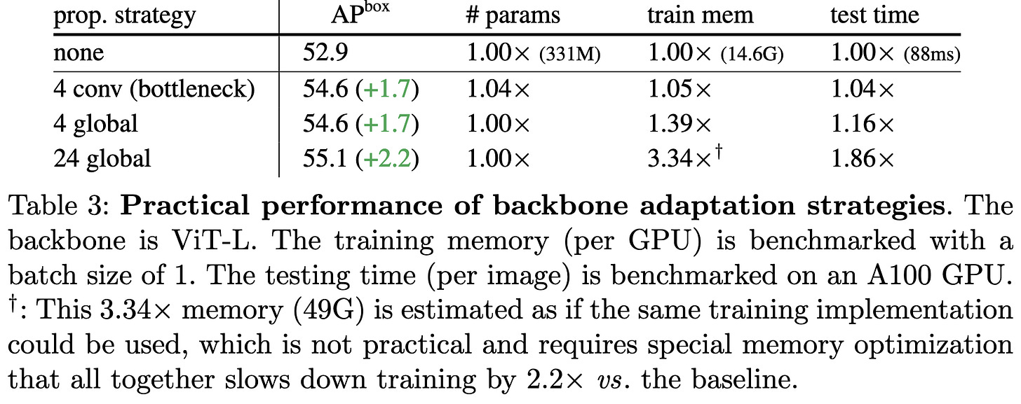
They then present various ablations on how to share information across windows, which turns out to matter quite a bit:
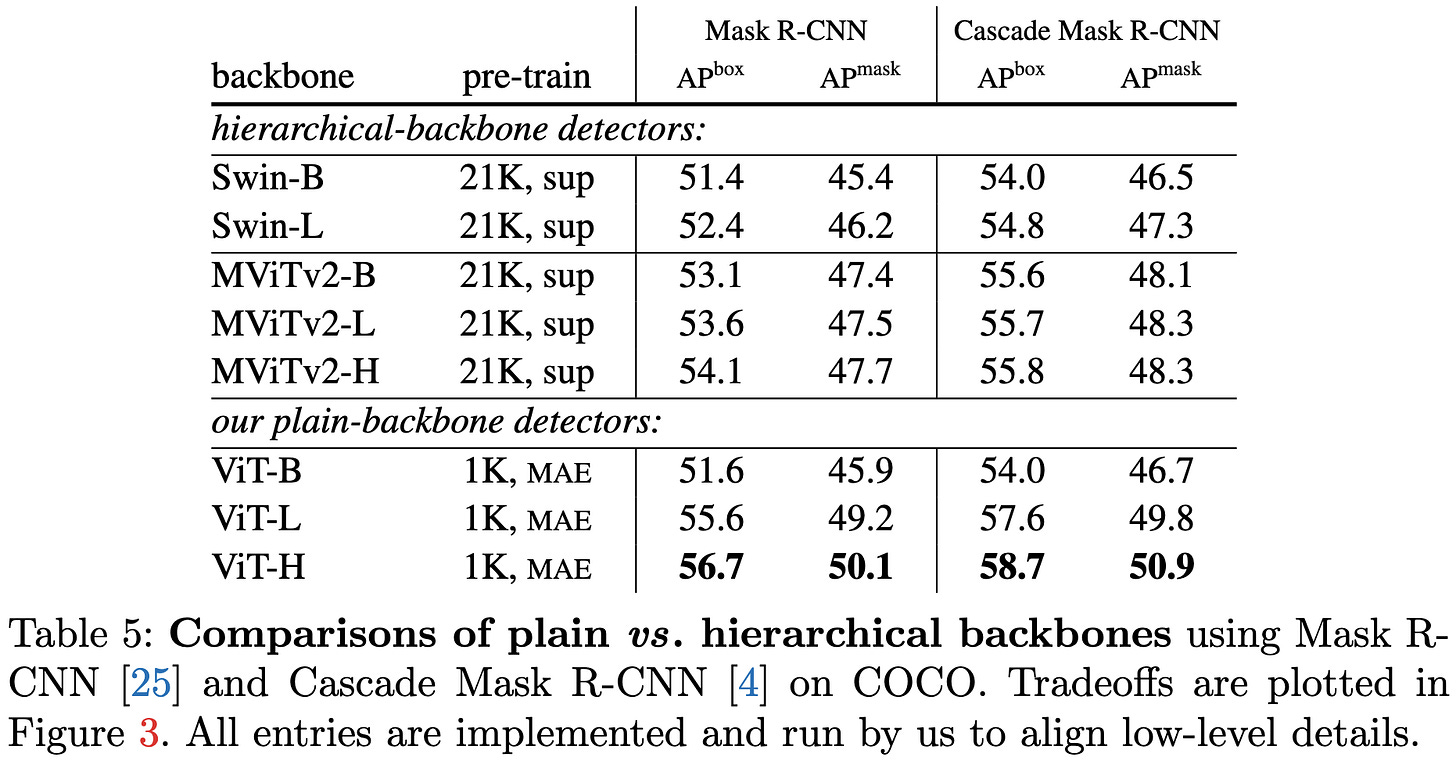
They find that the masked autoencoding objective is much more effective than supervised pretraining—so much so that ImageNet1k with MAE beats ImageNet21k supervised.
Partially because of MAE’s superiority, they’re able to beat previous approaches with their simpler backbones:
This is one of those paper to go through and read really carefully if you’re trying to max out object detection performance, since it threw a ton of compute at this problem in a lot of well-executed experiments.
Insights into Pre-training via Simpler Synthetic Tasks
Instead of pretraining on real text, you can get most of the benefit by pretraining on simple synthetic tasks. It was already known that there exist synthetic tasks that work fairly well, but the surprising result in this paper is that really simple tasks—like just input deduplication—get you almost as much benefit as fancier ones.
They find that the best fancy synthetic task is LIME (not the interpretability method—a symbol binding problem). But the best simple synthetic task is deduplication (“Set”).
Moreover, there are a lot of simple tasks that work pretty well.
Even transferring the learned means and variances for each layer to a fresh network is suprisingly effective.
One caveat here is that there’s not much benefit to using synthetic tasks—the authors find that training on real text gets at least as much benefit per sample.
But it is super interesting that such simple tasks works so well. I wonder how close to real performance one could get with a collection of simple tasks embodying different functions / reasoning primitives. Like, what if you taught it to do every function in NumPy? I’m not sure we could beat text data, but I wouldn’t be surprised if we could construct a complementary dataset that tends to lift accuracy when combined with a large text corpus.
Mask DINO: Towards A Unified Transformer-based Framework for Object Detection and Segmentation
Adds a mask to DINO and gets new SotA on COCO instance segmentation, COCO panoptic segmentation, and ADE20k semantic segmentation.
Language model compression with weighted low-rank factorization
Proposes using a weighted SVD when factorizing weight matrices, with the weight of each row equal to the sum of the estimated Fisher information for each parameter in that row.
Works better than raw SVD, but probably not a net time vs accuracy win. The way to see this is to note that cutting the rank in half is where you break even in FLOPs (but with 1.5x the data movement), so you’d need identical accuracy at a much lower rank to start getting a speedup.
Also note that fine-tuning will probably close this gap; in my experience, the initialization of factorized layers stops mattering as you train the resulting parameters for longer.
But still, an elegant problem formulation based on simple intuition.


