2022-9-18 arXiv roundup: Reliable fp8 training, Better scaling laws, Different minima are often just different weight permutations

This newsletter made possible by MosaicML.

---

FP8 Formats for Deep Learning

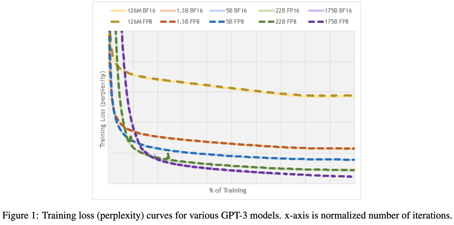
A group of NVIDIA, ARM, and Intel researchers got fp8 training working reliably, with only a tiny accuracy loss compared to fp16. This is a big deal for whether you should buy NVIDIA’s new GPUs, as well as for model export / MLOps workflows.

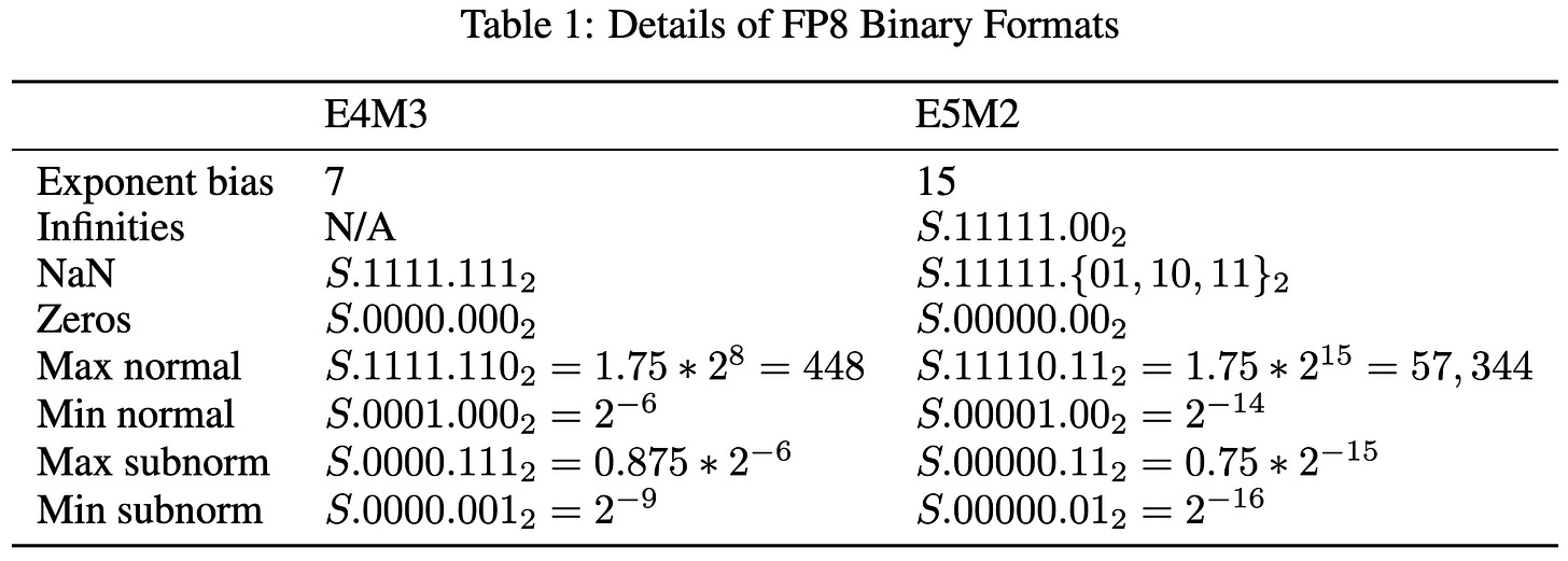
Methodologically, there’s not much that wasn’t present in these two papers. The one difference is reducing the number of NaN/Inf encodings in fp1-4-3 down to just one bitstring. In case you haven’t memorized the details of IEEE-754 floating point, usually all values with a certain prefix are considered NaN, wasting a bunch of possible bit strings.

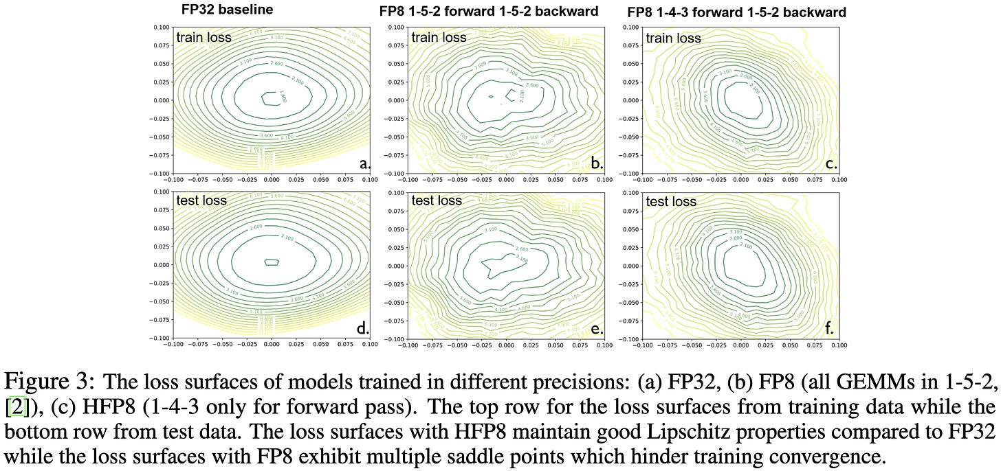
They use 4 exponent bits and 3 mantissa bits in the forward pass, and 5 exponent bits and 2 exponent bits in the backwards pass. They only cast the input operands for linears and convs to these formats—not the outputs or any inputs to elementwise operations. They also do channel-specific scaling for weights and tensor-specific scaling for activations. These choices mean they won’t get acceleration for most bandwidth-bound ops and will pay some overhead for the compute-bound ones, but they should get to spend most of their time in fp8 given sufficiently wide layers.

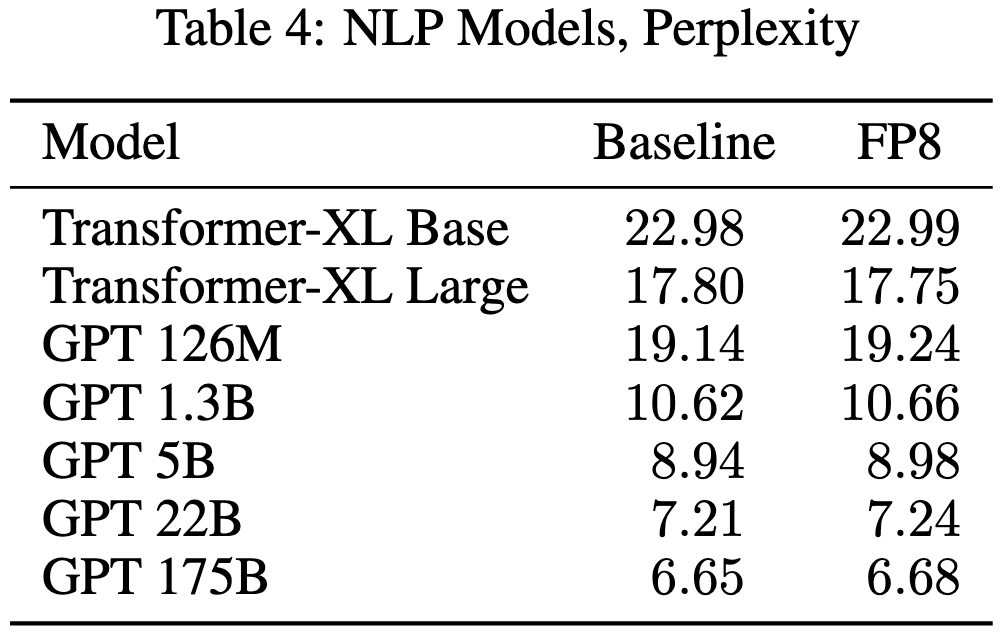
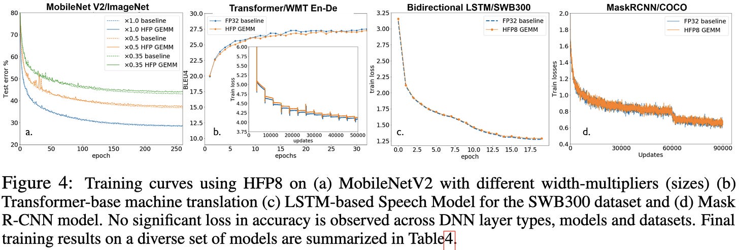
The big question is: how much accuracy loss does this approach cause? They find that, across a huge array of models and tasks, the consistent answer is: not much—around 0-.3% accuracy/BLEU/perplexity:

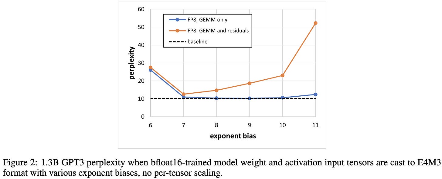
The accuracy does seem to plummet if you deviate from this exact quantization approach though. E.g., they find adding quantization of just the residuals yields big accuracy drops.

The other big result is that they can just convert from fp16 to fp8 models after training with no loss in accuracy. In fact, they consistently gain accuracy, which is a little weird and makes me worry about their baselines.

But the big inference use case here is skipping fp16 training entirely. If you do both training and inference in fp8, you save a huge amount of operational complexity. No weird deviations between what the data scientist saw and what happens in prod, no quantization-aware-training, no separate inference optimization team, etc. You just serve what you train, modulo math-equivalent optimizations like fusions.

These results are great news for NVIDIA’s upcoming Hopper cards. They already accelerate these fp8 formats 2x compared to fp16, and their “transformer engine,” while not described in much detail, might (?) help with the channel- and tensor-specific scale factors. So even though Hopper fp16 FLOPS/W and FLOPS/$ aren’t much higher than Ampere, effective FLOPS/W and FLOPS/$ might double.

There is the reality that most users won’t know enough to opt into fp8, but with tools like Composer becoming increasingly popular, that might become less of an issue over the next couple years.

---

Out of One, Many: Using Language Models to Simulate Human Samples

Similar to another paper we saw recently, they use GPT-3 to simulate human responses in social science experiments. But rather than try to replicate psych studies, they try to replicate the population-level statistics about behaviors and attitudes.

The clever idea here is including backstories in the prompts, with backstory demographics matched to the target population. E.g., the correct fraction of backstories will be from men vs women, liberal vs conservative, etc.

This turns out to work great. Given the right backstory distribution, the distributions of GPT-3 completions for voting patterns, religious observance, demographic information and more match the true statistics way better than chance.

I’m not sure yet what the implications of this are. But I hope that one is a partial story for alignment. If we can just add “I’m a nice person” to the prompt to get “nice” output, that would be an easy win.

I could also imagine designing prompts to get better results by forcing a model to consider multiple perspectives (e.g., “an Oxford professor would say that the answer is:”, followed by “but a farmer in India might say:”).

Or maybe, rather than a “better” answer, this will become a standard practice for internationalization and localization in ML-powered software. Like, if the user is an 18-25 year old in Brazil, prompt their autocomplete model with, e.g., “an 18-25 year old in Brazil would respond:”.

---

---

Test-Time Training with Masked Autoencoders

If you have a train vs test distribution shift, it might be worth continuing to update the model at test time. But you don’t usually get labels at test time, so your adaptation has to be unsupervised.

What they propose is finetuning the model with a masked-autoencoding objective to reconstruct masked-out patches of the test image. They do this finetuning for some number of steps, and only then make a prediction.

In more detail, they start with a pretrained encoder, a pretrained decoder, and a ViT model to make class predictions. The ViT model takes the output of the encoder as input, and is the only part they train on their training set. They tried training the encoder but, somewhat similar to locked image tuning, found that keeping the image encoder frozen worked the best.

Adding this domain adaption step before each test-time prediction definitely helps accuracy on corrupted versions of ImageNet images.

The main downside is that they do a bunch of training steps for every image at test time. There’s no reuse here—they reset to the pretrained model before every prediction. Though I suspect one could just finetune on the test distribution once to avoid this per-sample overhead.

These results bolster the case for continual learning, suggesting there are accuracy lifts to be had even when the data distribution qualitatively changes, rather than just becoming stale.

---

Efficient Quantized Sparse Matrix Operations on Tensor Cores

They accelerate a certain form of structured sparsity on modern GPUs through careful algorithm design and kernel writing.

The basic observation they exploit is that tensor cores can operate on strided tiles, as long as they’re contiguous on their last dimension. So you if have groups of 8 contiguous nonzeros, you can pack all the nonzeros together and do a smaller “dense” matrix product.

They apply this observation to matrix products with one sparse input matrix (SpMM, above) and with sparse outputs (SDDMM, below).

Their matmuls become faster than dense f16 at 50-70% sparsity, depending on what bitwidth they use. I’m not certain they really beat int8 quantization though; they show cuBLAS int8 as one of their baselines, but for some reason it’s slower than cuBLAS f16, which is weird.

They do show end-to-end latency gains for sparse transformers.

And mostly preserve the transformer accuracy. Although, again, I’m not sure this beats int8 quantization.

Regardless though, people pushing the limits of efficient sparsity and (not to mention conducting thorough evaluations) are providing valuable datapoints about what’s possible in this area.

I had to skip over most of the method because it’s super dense, but I just wanna commend them for doing a great job of illustrating everything. This is extra impressive because their proposed method is big and detailed, covering everything from data layouts to memory bank conflicts to fast transposes to prefetching.

If you want to gain appreciation for how ridiculously easy most deep learning research is compared to hardcore systems work (from a conceptual, background knowledge, and implementation perspective), take a look through this paper. And if you know anyone who works on stuff like this, give them a hug because they probably need it.

---

Revisiting Neural Scaling Laws in Language and Vision

A whole bunch of clear thinking about scaling laws, from which they derive better alternatives to common practices.

First, they point out that a scaling law that interpolates between sizes you’ve seen is way less valuable than a scaling law that lets you extrapolate to larger sizes. But most of the scaling literature focuses on the former, reporting “fit” based on the training set rather than held-out sizes. And sadly, the scaling exponents can be significantly different in these two cases.

Next, they consider a simple problem: logistic regression on a synthetic binary classification task with a known Bayes error rate (lower bound) and random guessing error rate (upper bound). They show that existing scaling law estimators don’t account for the random guessing error rate and do poorly unless you throw away that part of the curve.

To fix this, they propose a new parametric form for scaling laws that handles an initial error rate but asympotically becomes a power law. Namely, they set the reducible error over the already-reduced error equal to a power law. Plus there’s another free parameter α that apparently improves the fit.

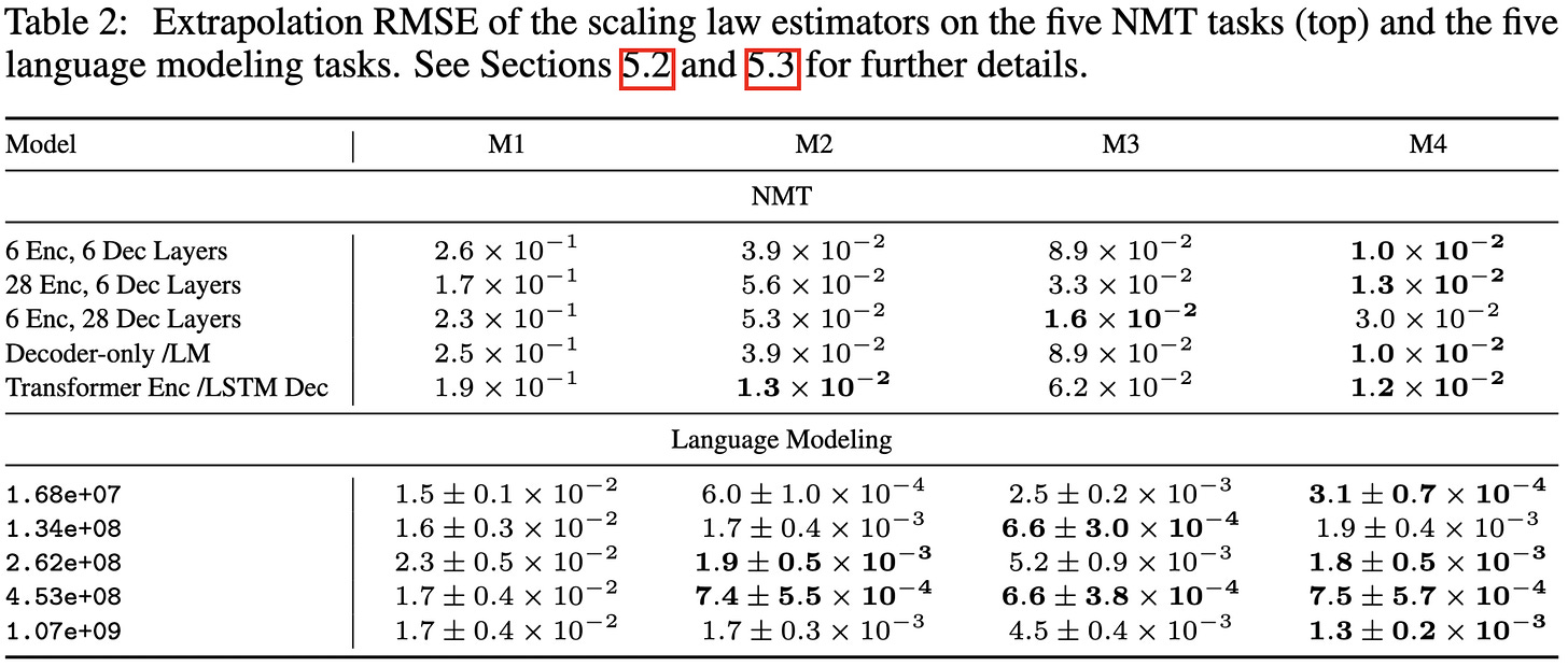
This parametric form improves the fit when extrapolating across all sorts of vision and language tasks.

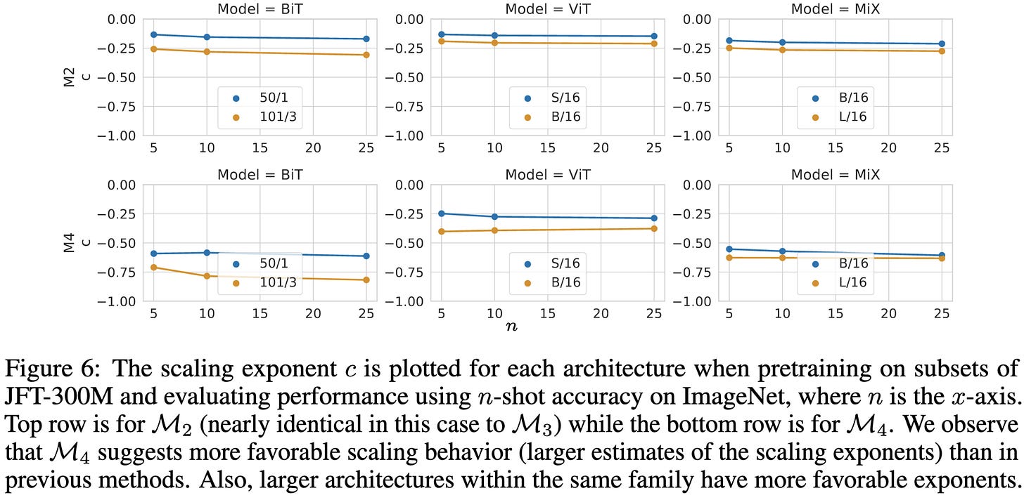
Interestingly, for image classification, they find better scaling with respect to dataset size (bottom row) than the vanilla power law predicts (top row).

They also find decreasing returns to dataset size as models grow larger in language modeling. This differs from their flat image classification curves, but is consistent with the predictions from the more typical power law + noise floor parametrization.

This definitely gave me clearer thinking about scaling laws, but also made me suspect we still don’t quite have the right parametrization yet. Their improved results convinced me that other formulations aren’t ideal, but their extra α parameter and loss-reduced-so-far denominator seem unintuitive enough that I also doubt theirs is ideal. That said, reality need not be “intuitive,” so it could be that their equation has nailed it.

---

SmartKex: Machine Learning Assisted SSH Keys Extraction From The Heap Dump

If you can get access to a process’s memory, you can use simple ML to quickly identify likely SSH keys. It’s already possible to find keys by brute force, but the ML makes it much faster.

You’re probably already pwned if an adversary can inspect the contents of your RAM, but I could imagine interesting threat models around “secure” connections to / sandboxing of malicious AI (resulting from data poisoning, RL gone horribly wrong, etc).

---

Diffusion Models in Vision: A Survey

What the name says. Does a good job of describing lots of methods and tabulating which models and datasets different papers use.

---

Random initialisations performing above chance and how to find them

Are all neural network minima the same, aside from permutations of the weights within each tensor? Apparently, yes—at least sometimes. Their experiments both flesh out this conclusion and show some surprising implications.

First, they find that the loss barrier between one network’s solution and the permuted other network’s solution 1) is small, 2) decreases with width, and 3) increases with depth. This is evaluated on small MLPs trained on CIFAR-10-scale datasets.

Next, they show on the same tasks that different initializations lie in the same loss basin. What demonstrates this is that taking two random initializations, permuting one to match the other one, and then averaging the two consistently has good test accuracy (left subplot). As in, with no training, you can just average initializations and get out a way-better-than-chance model.

You can even average more random initializations to get better accuracy (middle), although there are sharply diminishing returns past two for wide, shallow models.

These results don’t always hold for CNNs. Accounting for the permutation does lower the loss barrier a lot, but at high learning rates, CNNs seem to converge to different minima.

Another promising contribution they mention in Appendix B is a means of finding good permutations to match up the networks without any training. Basically, they find a permutation that aligns the line segment between one initialization and the permuted other initialization with the direction of fastest decreasing loss, such that the halfway point is a minimum.

The experiments are small scale and I’m not certain about the details of how they’re finding permutations, but the results are super interesting. A well-designed science-of-deep learning paper and I can’t wait to see someone try to replicate this at larger scales.

---

Git Re-Basin: Merging Models modulo Permutation Symmetries

Another exploration of linear mode connectivity after correcting for permutations of the weights, with a bunch of cool contributions.

First, they describe three algorithms for finding a permutation that aligns the weights of two different networks. One is based on ordinary least squares on the activations + linear assignment; one is based on aligning the weights directly with no data; and one is based on learning the permutation via gradient descent and the straight-through estimator. The first two are fast but the last one works a little bit better.

Next, they show that there exist simple problems for which linear mode connectivity doesn’t hold. They do this via a constructive proof involving a binary classification problem and a 2-neuron single-hidden-layer MLP.

In terms of results, they somewhat contradict the previous paper.

Their first contradictory finding is that MLPs with different random initializations *aren’t* in the same loss basin at the start of training. Or at least, they can’t find a permutation that aligns them.

Second, with wide enough ResNets, they find that there’s essentially no loss barrier on CIFAR-10 between completely separate models once you align them with a good permutation. This might contradict the previous paper if they used large learning rates, though they also confirm that there is a barrier at the original width. Consistent with the previous paper, they find that wider models tend to have lower loss barriers.

Perhaps their most surprising result is that you can train two models on disjoint subsets of CIFAR-100 with different class distributions and then merge them together post-hoc, as long as you permute one of them well.

It’s rare to get two papers in one week with such closely-matched experiments. And it’s great—you get to view the results of each paper with memories of the other still fresh. This pair of papers, along with branch-train-merge, model soups and this model soups follow-up, suggest to me that we can probably merge separate models productively—at least if we either start them all from the same pretrained model or (more excitingly) just figure out a permutation to align them.

---

On the Factory Floor: ML Engineering for Industrial-Scale Ads Recommendation Models

A detailed Google paper about lessons learned regarding huge RecSys models. This is less “here’s our method” and more, “here’s a whirlwind tour of years’ worth of findings.” Some highlights:

• They use sparse ngram features fed into MLPs; no transformers

• They need to handle over 100k queries per second

• Calibration on individual samples matters, not just populations. You have to get the clickthrough probability right for this ad to bid properly. They handle this with an extra loss based on Langrange multipliers.

  

• They’re doing continual learning, evaluating using live traffic and then training the model on what the user actually clicked on.

• Factorizing huge matrices provides a speed vs accuracy improvement, though only if you also scale up the layers. They got 7% faster training steps at iso accuracy this way.

• They care a lot about reproducibility because 1) they care about small differences and want to know if some new model is actually better, and 2) reproducibility is especially hard in a continual learning setting like theirs where your predictions influence your observations (i.e., which ads the user sees).

  • They actually choose stuff like their activation function (SMeLU) to minimize cross-run variance.

  • For the same reason, they start with a simple loss function and gradually add stuff like distillation + ranking losses.

• At iso inference latency, ensembles consistently work worse than single models.

• Using Distributed Shampoo helps a lot. At least once you add a momentum term and graft in AdaGrad’s lr schedule.

  

• They have separate model components for evaluating an ad’s content and its placement on the screen.

  

• They do neural architecture search by training one big supernet and having an RL-based controller sample + eventually select a subnetwork.

Overall, they found a bunch of techniques that improve training time, inference latency, and accuracy better than simple baselines like scaling up the model:

The biggest decrease in training cost comes from intelligent data subsampling. This is partly throwing away old data and partly downsampling the (far more frequent) negative samples to obtain class balance. They especially downsample data from ads the user likely didn’t see or that the distillation teacher model thought were least likely to be clicked.

Always great to get a glimpse into the problems and solutions of what is probably the world’s most mature machine learning organization.

---

Hybrid 8-bit Floating Point (HFP8) Training and Inference for Deep Neural Networks (2019)

They train neural nets in fp8. Weights and activations use 1 sign bit, 4 exponent bits, and 3 mantissa bits (fp143), while gradients use 1 sign bit, 5 exponent bits, and 2 mantissa bits (fp152). The latter has more dynamic range but less precision within a given interval.

They find that, with the right software-level changes, they can train models in fp8 with almost no loss of accuracy. If you zoom in, you can see the fp8 lines slightly above the baselines, but it’s subtle.

One necessary change to avoid accuracy loss is smart handling of the output softmax. If you naively quantize it, multiple large elements will all get clipped to the maximum representable value, making their classes all appear equally likely. To fix this, you need to subtract off the largest value first and then quantize.

Two other fixes are a) updating the batchnorm variances using both running statistics and a quantization-aware formula they provide, and b) using f16 for depthwise convs. The latter have low output variance, which makes the quantization noise matter a lot more, and are also lightweight enough that using higher precision doesn’t hurt you much.

They also have to add a bias to the exponent when using fp143 to reduce the quantization errors. Although they also seem to do adaptive loss scaling to get the dynamic range of the gradients in the backwards pass as large as possible without overflow (similar to AMP).

With these fixes, they can can not just train or finetune models to full accuracy, but directly convert an fp32 to model to fp8 at inference time.

They also propose an algorithm for reducing the bitwidths of gradients when using their hybrid floating point training scheme.

They compute the gradients with an fp16 reduce-scatter, which leaves each worker with one slice of the gradient. Each worker then uses this gradient to update its slice of the weights. The workers then share their slices with everyone else in fp143. Each worker also tracks its running quantization error and adds that into its updates.

Probably the cleanest way to implement this is with sharded weights and optimizer states, with your allgather done in fp8 and optimizer modified to track elementwise residuals.

Using the above distributed training modifications, they manage to train models in fp8 with almost no accuracy loss on average.

This paper makes it seem like, with just a few software-level fixes, you can reliably train in fp8, which is super cool. However, 1) later work seemingly couldn’t get this same reliability, and 2) who knows if this is all the fixes that we need, or if there will be a long tail of model-specific interventions required.

---