

2022-10-30 arXiv roundup: 1 million GPU hours, Scaling laws, Science-of-deep-learning papers
2022-10-30 arXiv roundup: 1 million GPU hours, Scaling laws, Science-of-deep-learning papers

This newsletter made possible by MosaicML.
What Language Model to Train if You Have One Million GPU Hours?
They ran a variety of experiments on 1B to 13B parameter models to help them figure out how best to train their final huge model. We’ll go through the experiments one-by-one.
First, using diverse, high-quality datasets can significantly improve accuracy.

Next, they replicated Alibi as an attention enhancement. Consistent with our findings, it works great.
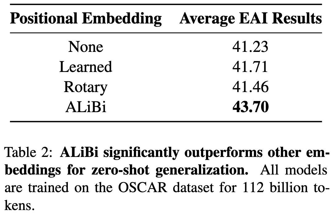
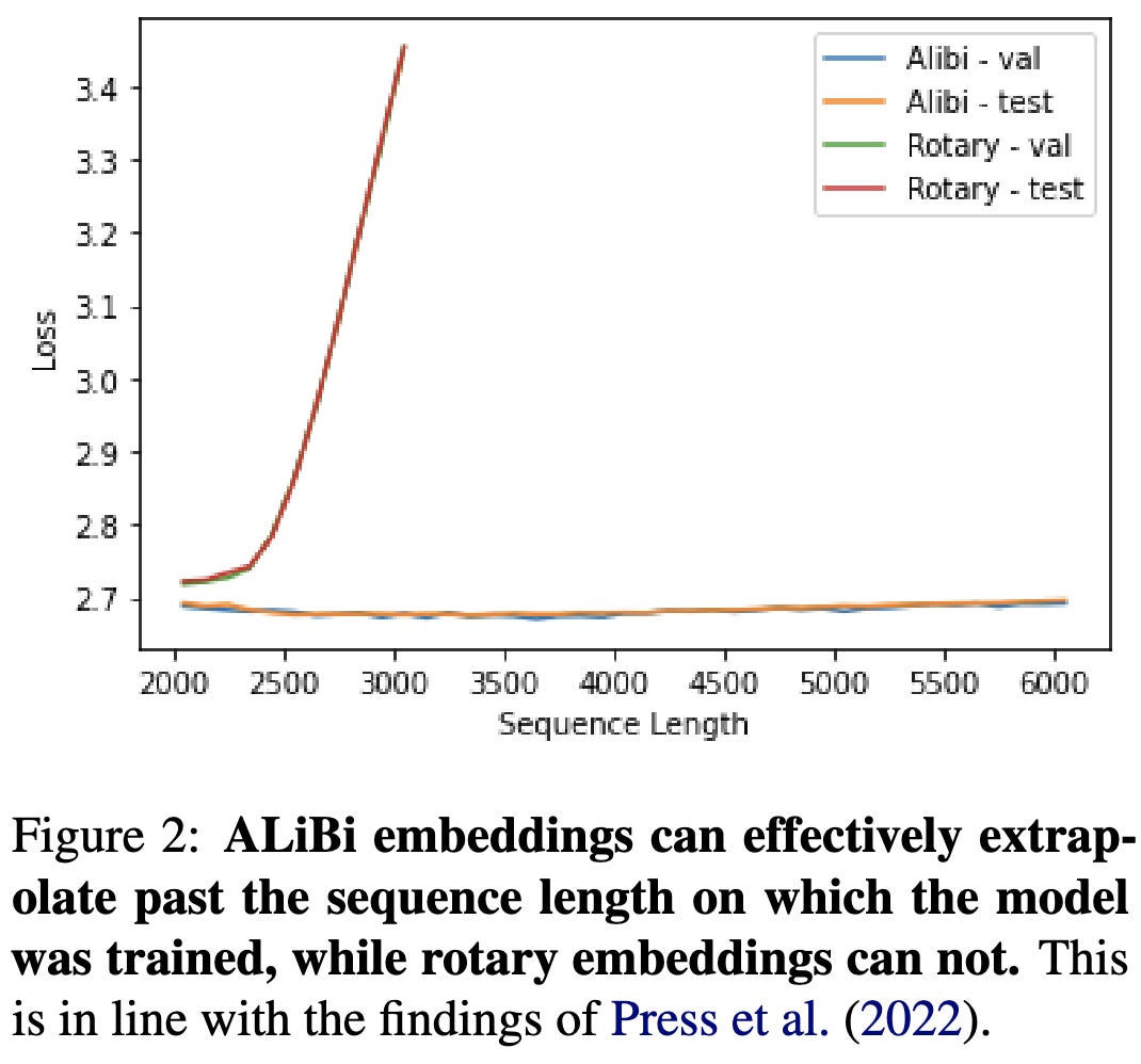
Alibi also allows extrapolating to lengths longer than those seen during training.
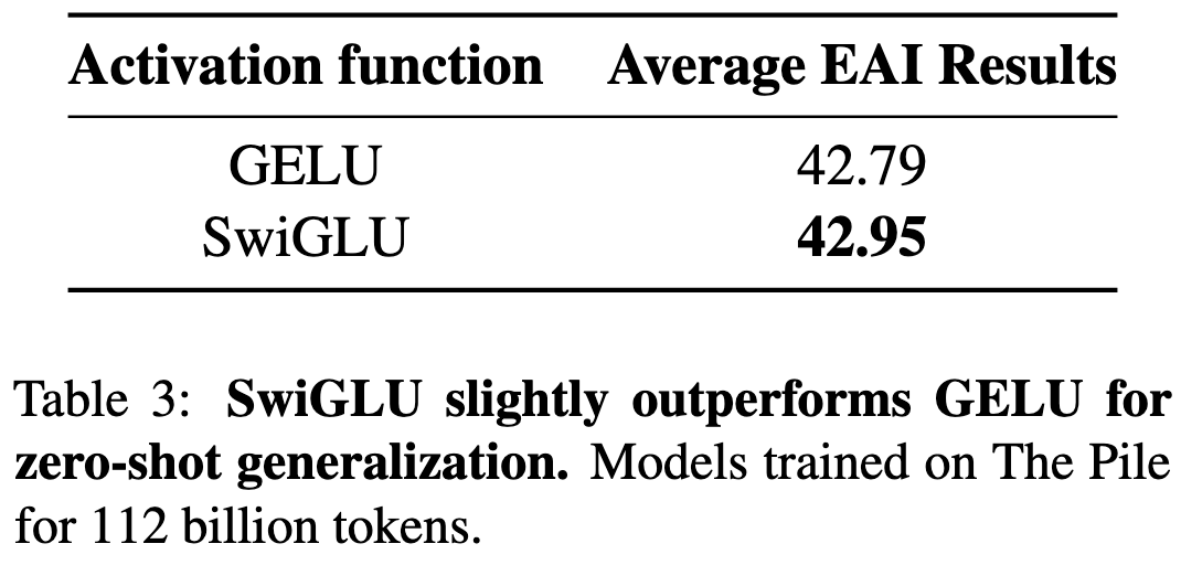
You can beat GELU by a little bit with SwiGLU.
Adding layernorm after the embeddings hurts accuracy.

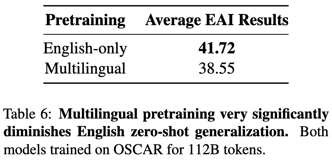
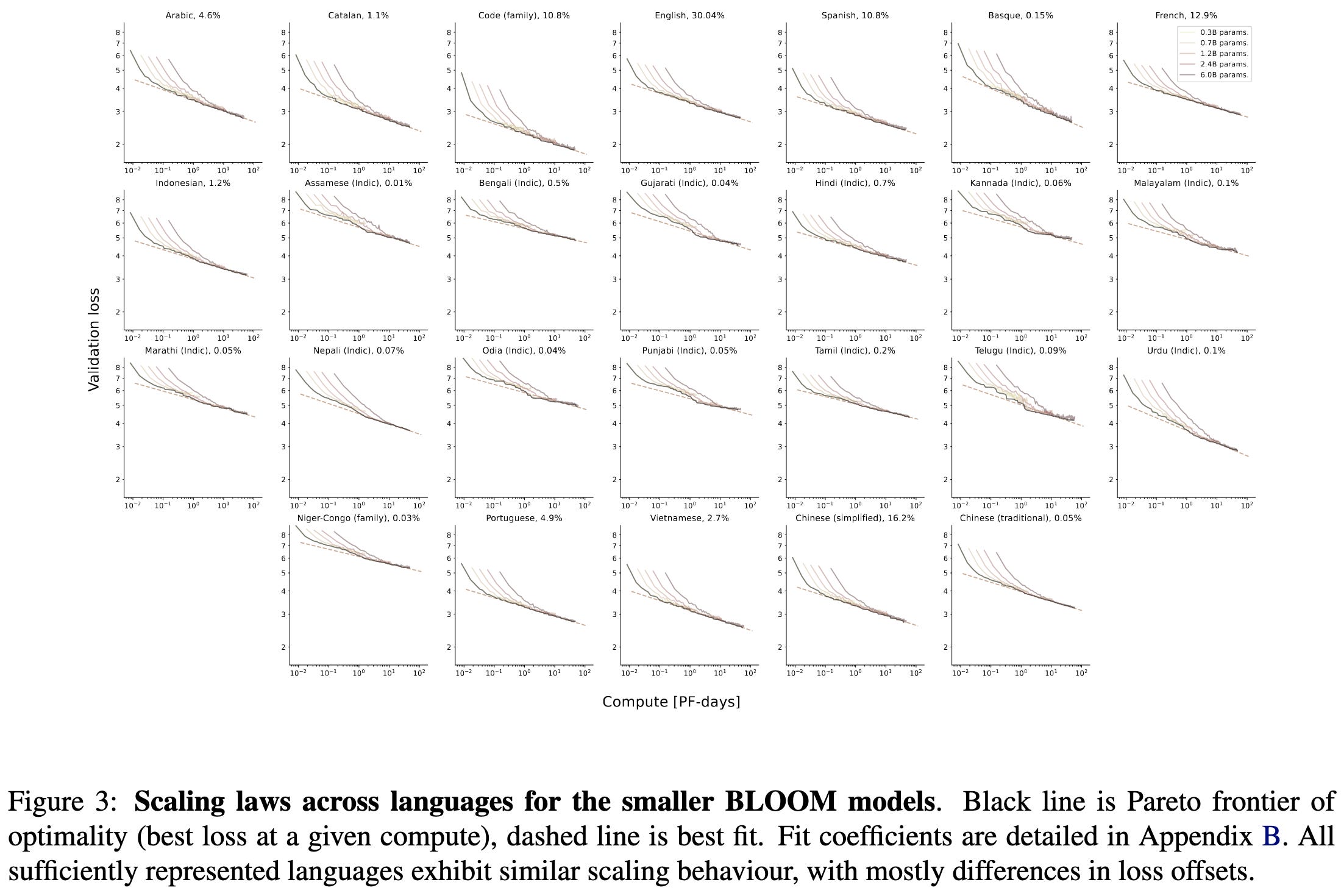
If you only care about English text, multilingual training hurts you quite a bit.
Different languages have surprisingly similar slopes in their optimal scaling frontiers.
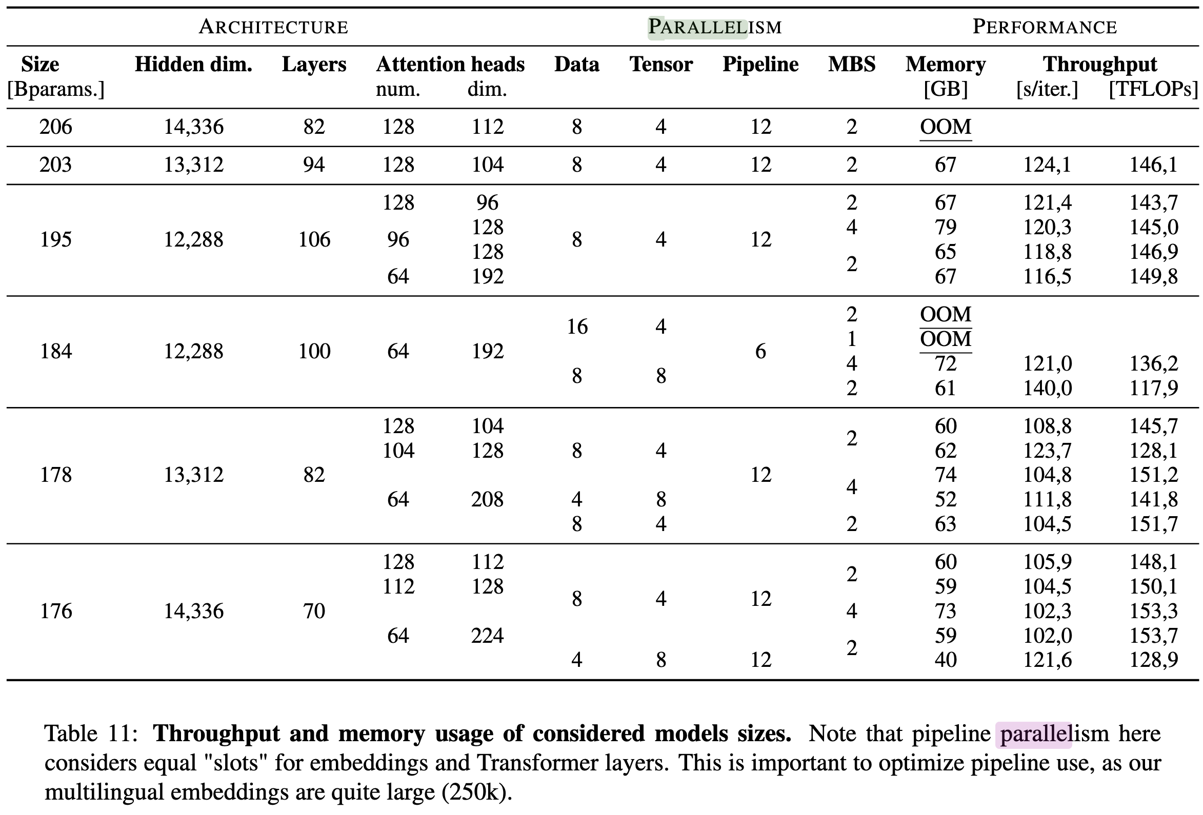
To get their final model, they microbenchmarked many different variants and went with the one that ran the fastest with the highest expected accuracy. Unsurprisingly, having side length 128 in your attention heads runs faster than 112 or 64.

To get the huge model to actually run, they forked Megatron-DeepSpeed and messed with different combinations of data, tensor, and pipeline parallelism.
Their final training run used around 400B tokens. This is way fewer than what the Chinchilla results would suggest, though they note that it’s kind of a moot point since they don’t have more data.
Relatedly, when not accounting for the learning rate schedule like in the Chinchilla paper, they reproduced the OpenAI scaling results. Always great to see important findings independently replicated.

They don’t really report any results using the final 176B parameter model, but they do have this nice table condensing all of their findings with smaller models.

The most interesting aspects of this to me are on a meta level. First, large scale deep learning is starting to look like chip design. In the hardware world, you test the crap out of your design before you actually write the huge check to fabricate it. Machine learning seems to be headed towards a similar workflow—only, at present, we don’t know how to “test your design” reliably.
Second, it’s interesting to see the amount of compute getting put into publicly-available models. Supposing they got their 48 8xA100 boxes for ~$16/hr each (2x cheaper than on-demand EC2 pricing), this is $2M of compute. This is way less than the big players use, but more than enough to train a GPT-3-quality model with the right infrastructure. Suggests a 2 year SotA → commoditized delay.
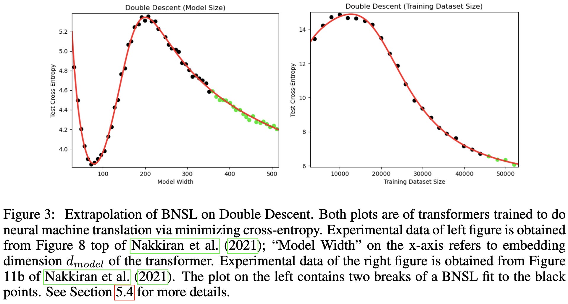
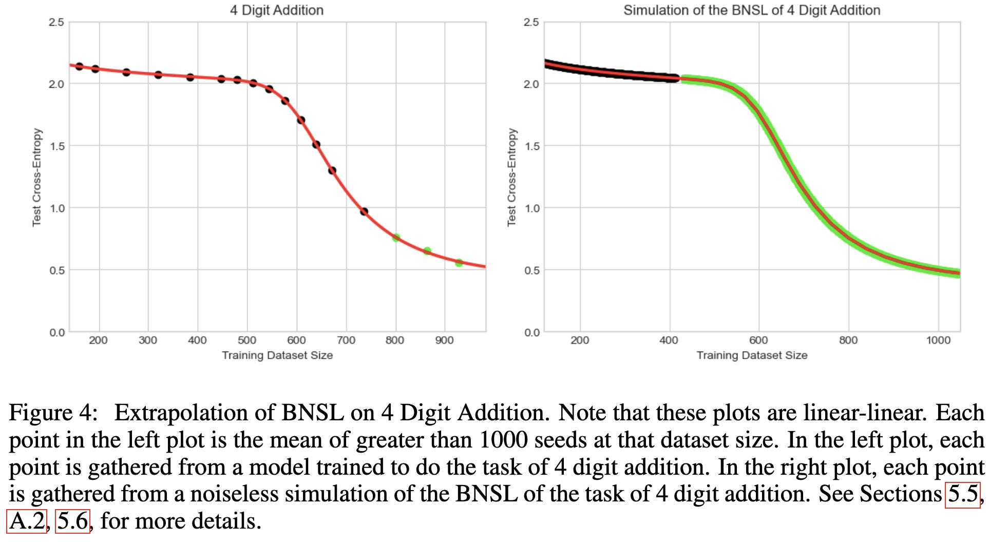
Broken Neural Scaling Laws
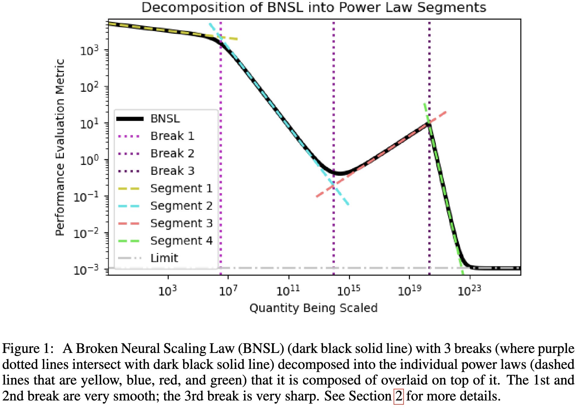
They fit a soft piecewise linear function on log-log axes, instead of a linear one (i.e., a power law). This lets them deal with phenomena like double-descent.
The exact functional form they use is below. It’s not actually hard piecewise assignment, and instead has different terms “kick in” at different values of x.
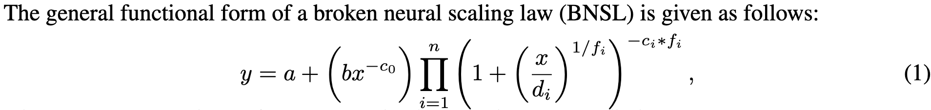
This functional form lets them fit scaling curves better than existing power law variants (named M1-M4).

These better fits hold across a variety of NLP, vision, and even RL tasks.
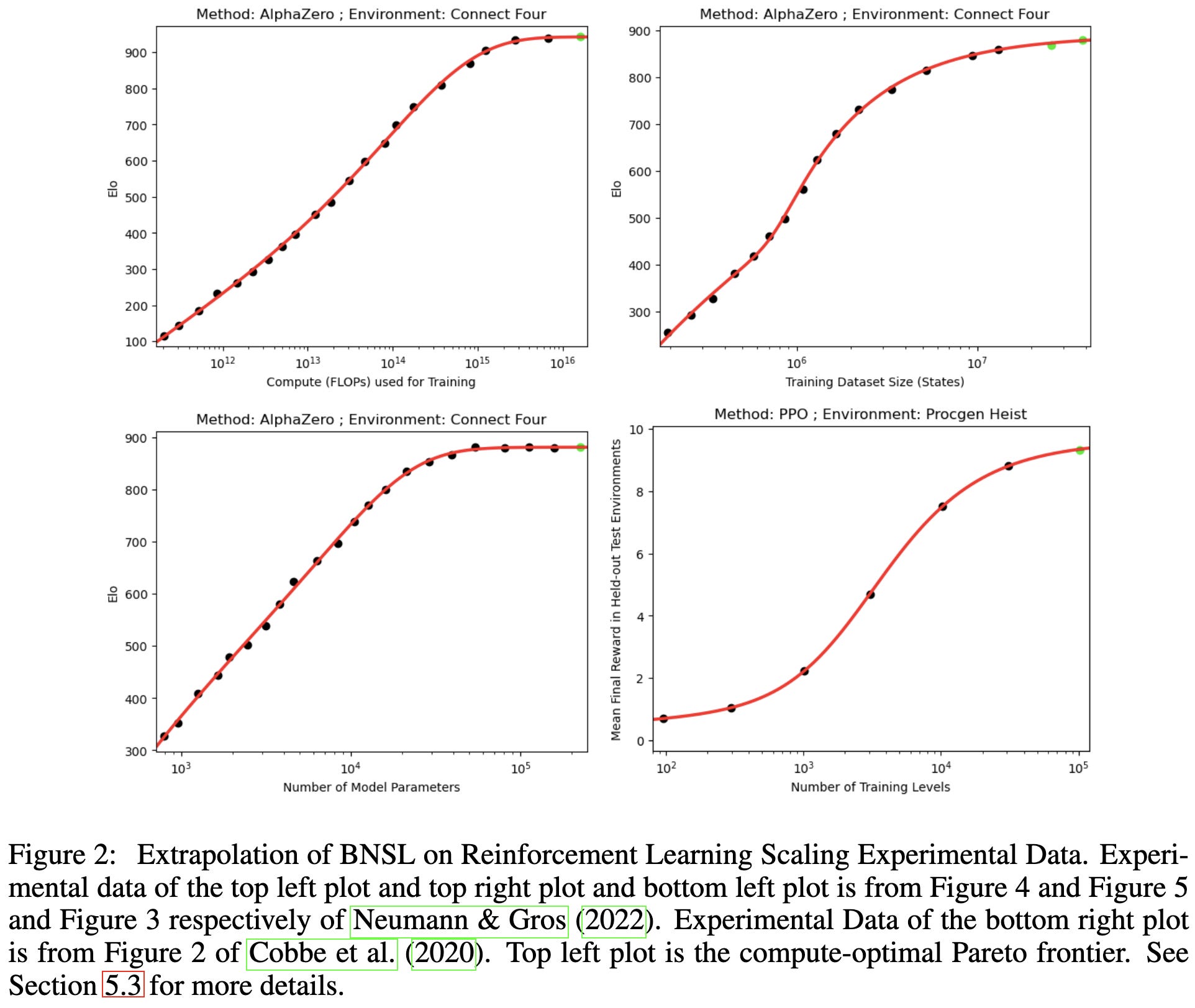
As intended, their method works well with weird scaling curves that seem to have multiple regimes.
I see two implications from these results. First, the finding that we can get better fits by adding more degrees of freedom—even with so few samples—suggests that maybe we should just be treating scaling curve fits as a generic time series forecasting problem.
Second, it suggests that either:
there isn’t a simple underlying “physics” giving rise to scaling laws, or
this “physics” includes some nuisance variables we don’t yet know about.
If the true dynamics were log-log linearity + noise, we wouldn’t be able to extrapolate better by fitting a fancier model like this paper does.
Scaling Laws Beyond Backpropagation
“There is never a regime for which the degradation in loss incurred by using [Direct Feedback Alignment] is worth the potential reduction in compute budget.”
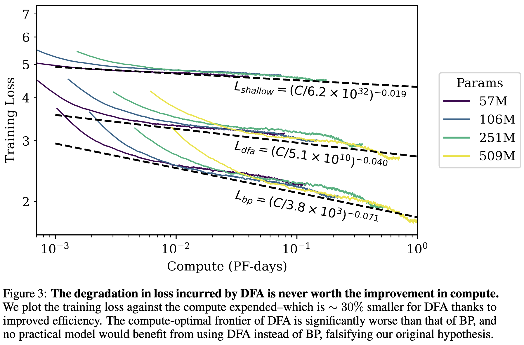
…at least as evaluated on large, decoder-only, causal language models.
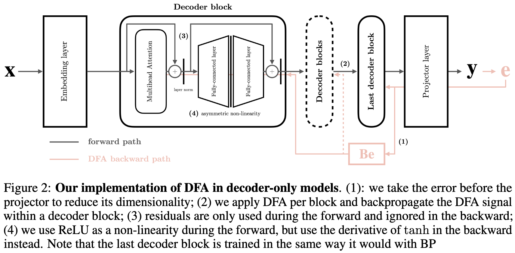
Part of me will always believe we can beat backpropagation, but boy is it hard.
Characterizing Datapoints via Second-Split Forgetting
Similar to Metadata archaeology and other work, they suggest inspecting samples based on how models perform on them over time. Unlike other work though, they recommend doing so by using a separate split of held-out data.

Concretely, they characterize each sample using the “first split learning time” (epoch after which it is never misclassified) and “second split forgetting time” (fine-tuning epoch after which it is never again correctly classified).
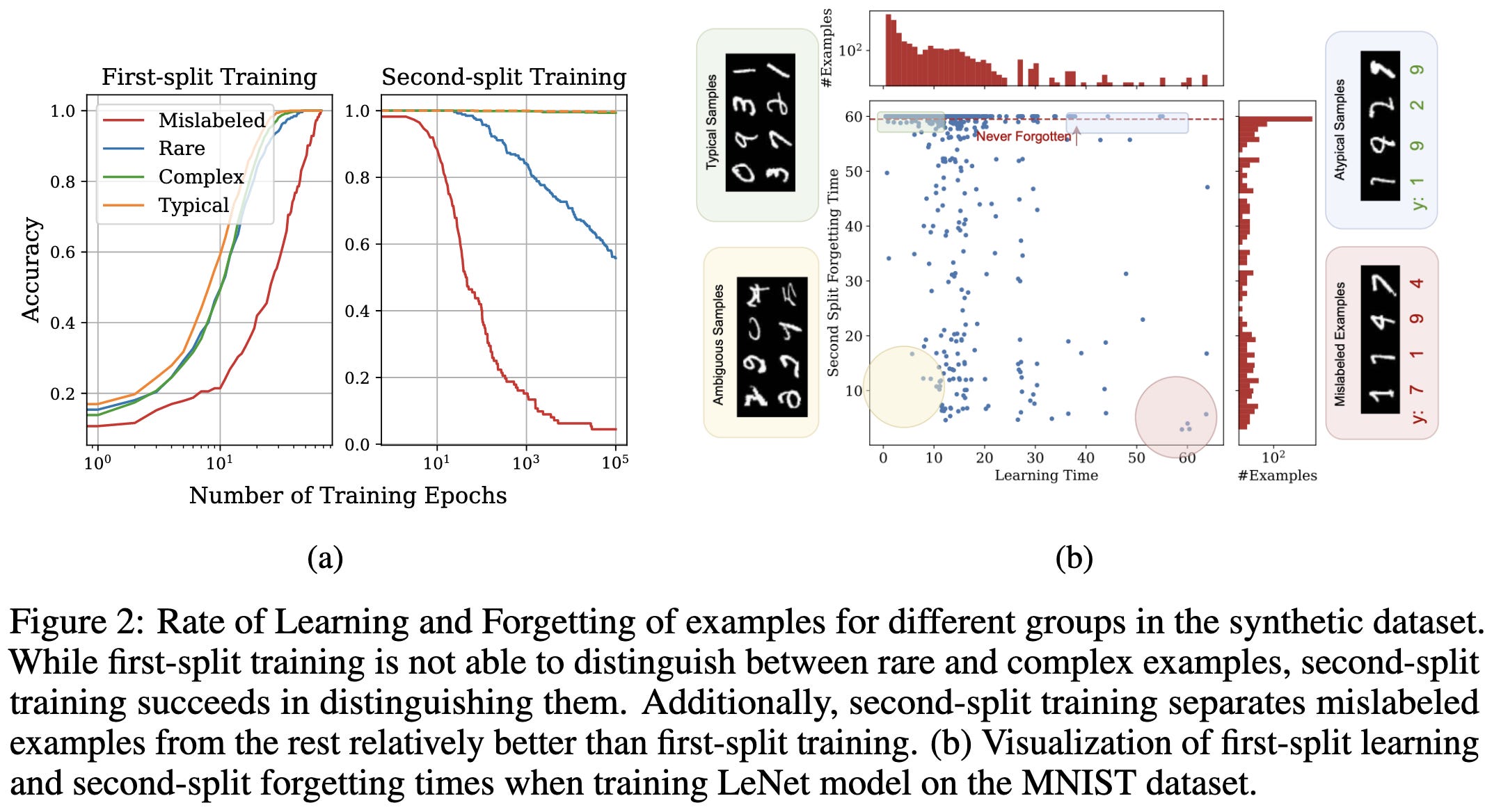
They find that the combination of these two scalar features works well for identifying mislabeled samples.
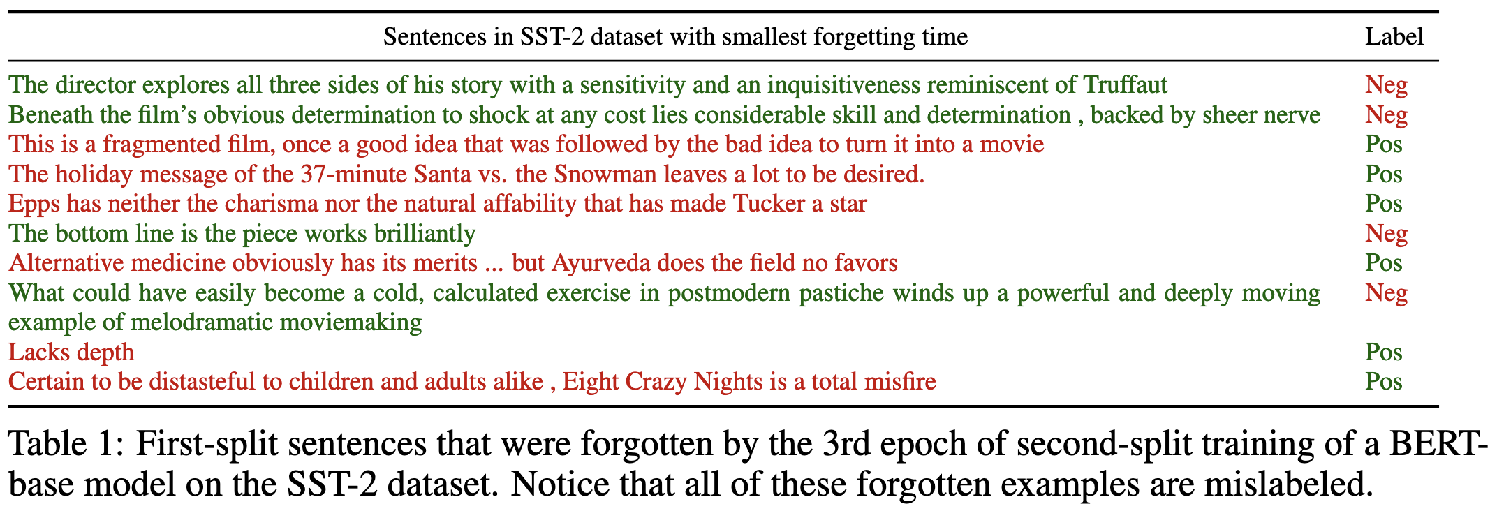
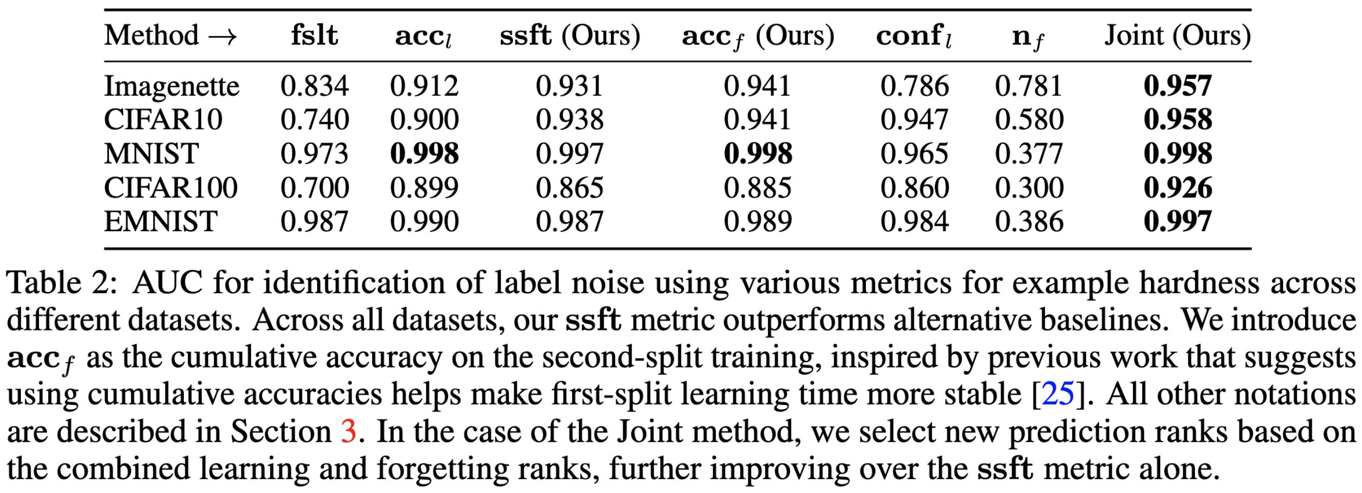
According to small-scale experiments, removing the samples that their method thinks are most likely to be mislabeled can increase accuracy.
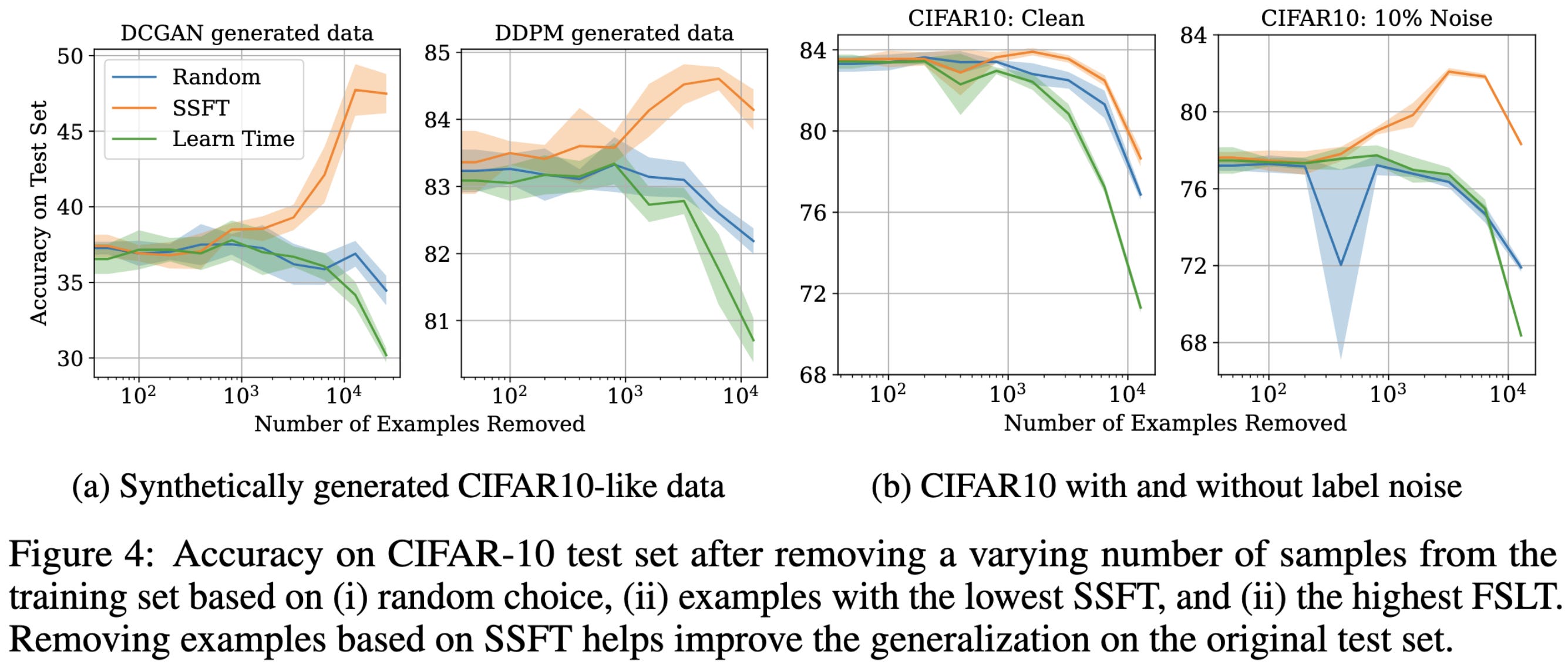
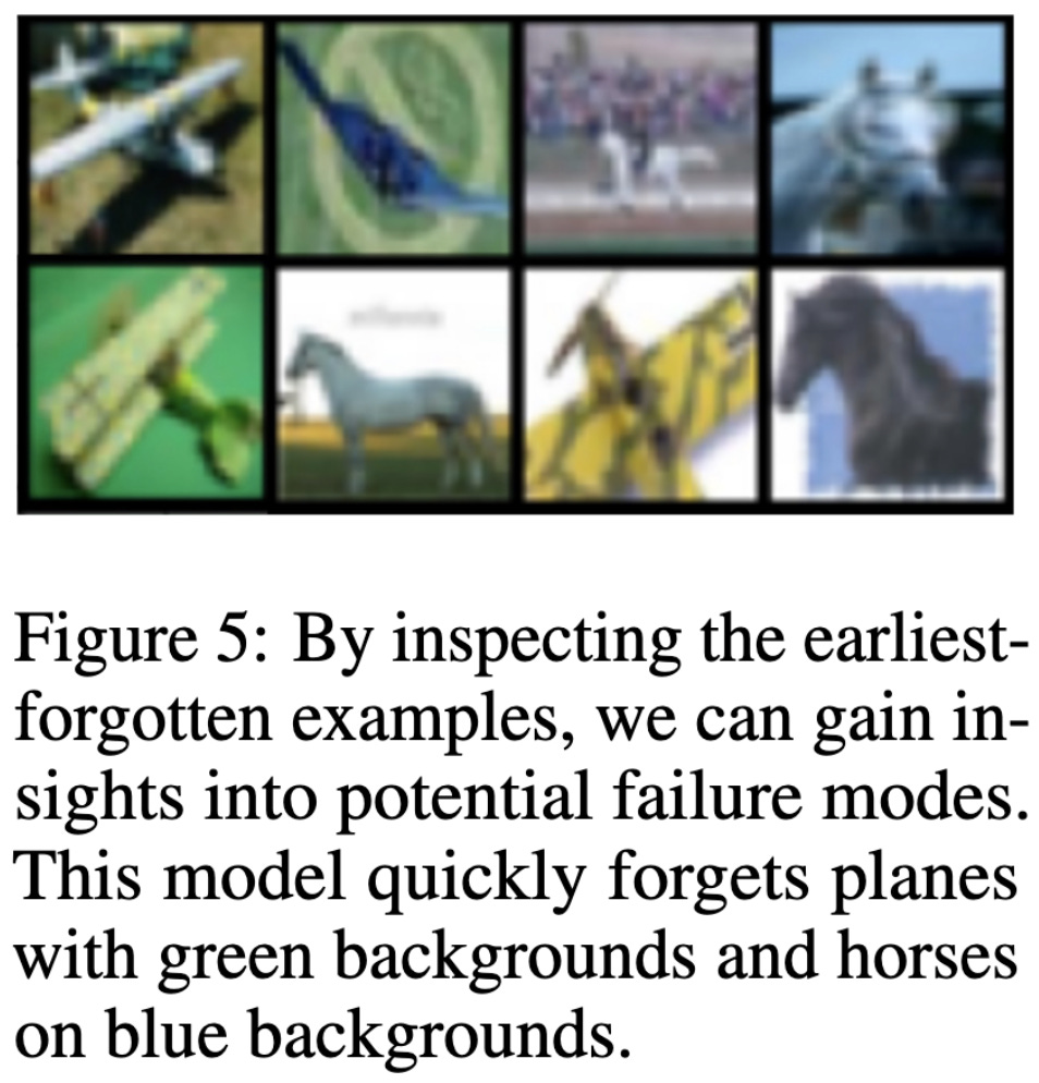
They also argue that looking at learning and/or forgetting time can be helpful for understanding model predictions and failure modes.
This is less of a tour-de-force than the metadata archaeology paper, which suggests that maybe using the full time series of predictions/losses is more informative than scalar features extracted from those time series.
But either way, I like their idea of computing forgetting statistics in addition to learning statistics. And it’s great to see more replication of learning/forgetting times being a useful feature for characterizing sample difficulty.
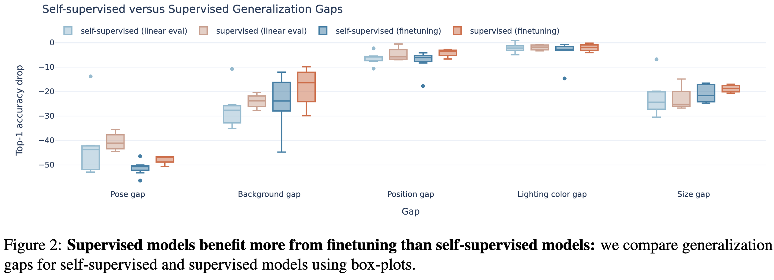
The Robustness Limits of SoTA Vision Models to Natural Variation
They used objects from Sketchup’s 3d warehouse rendered on various backgrounds to systematically study vision model invariances. Put simply, these models are not that invariant. Changes in pose, background, and size hurt accuracy the most.
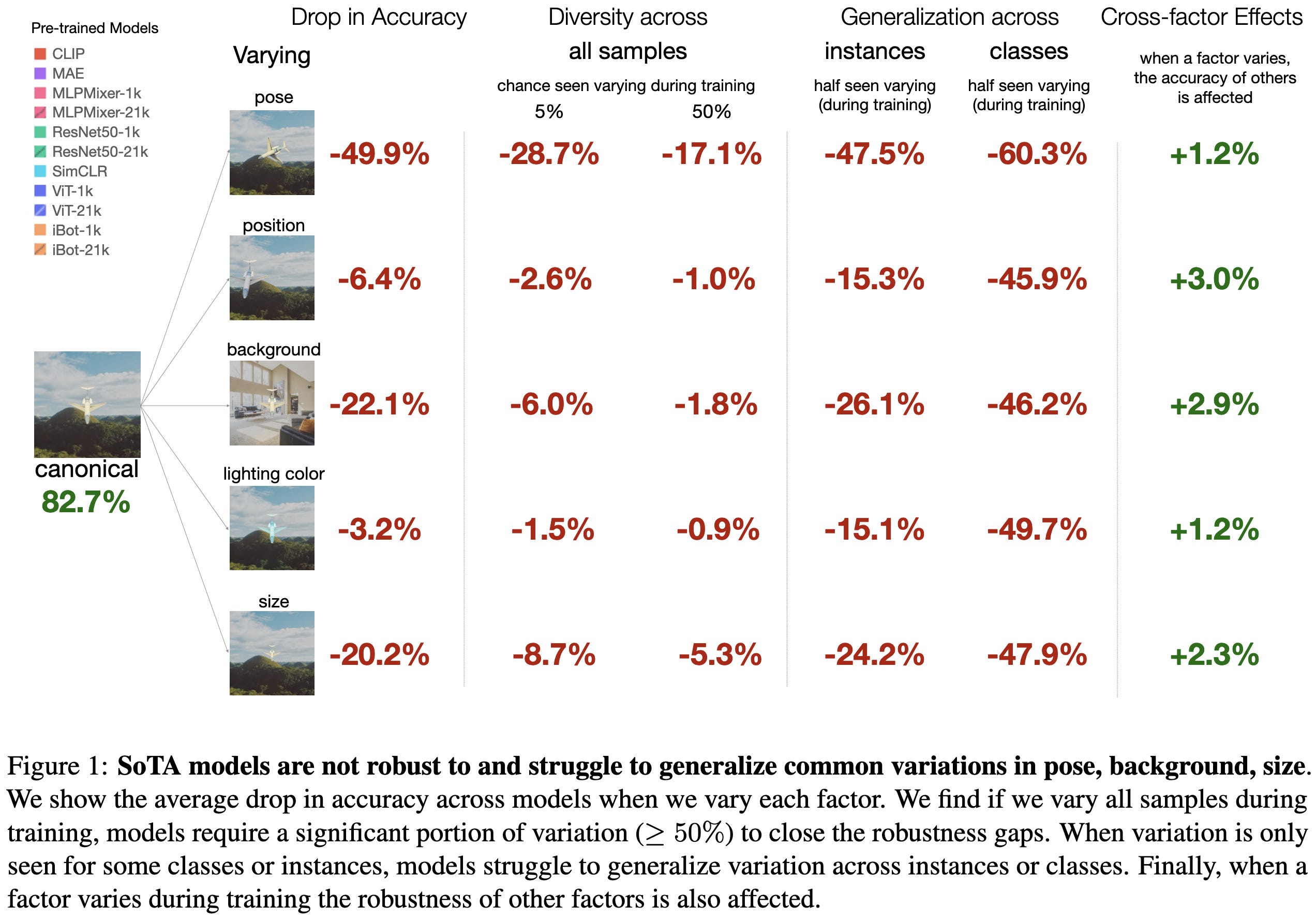
Different models and training approaches obtain different levels of invariance, though the relative impacts of different nuisance variables are fairly consistent across models.
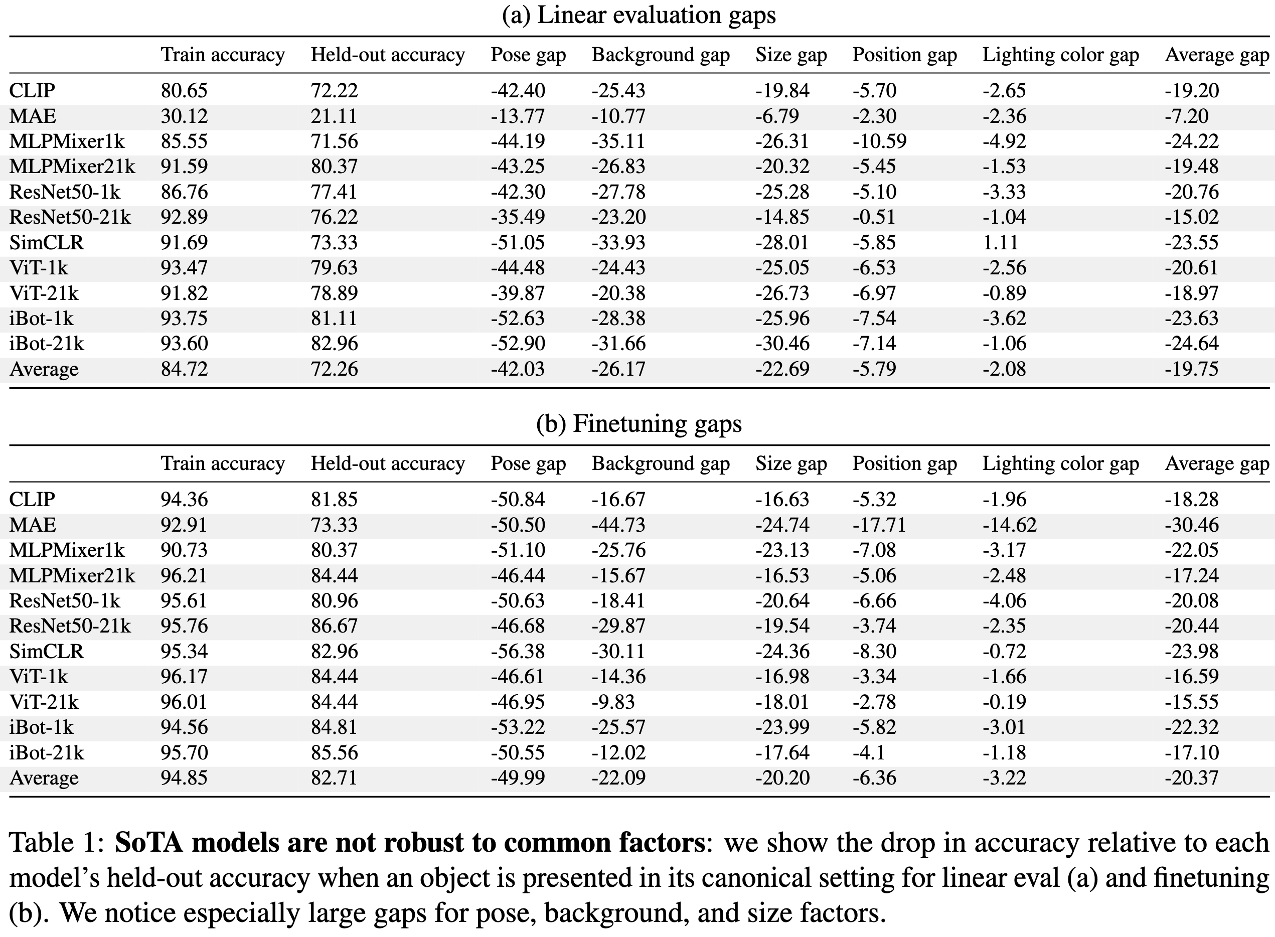
Supervised pretraining with finetuning tends to yield the lowest train vs test gap.
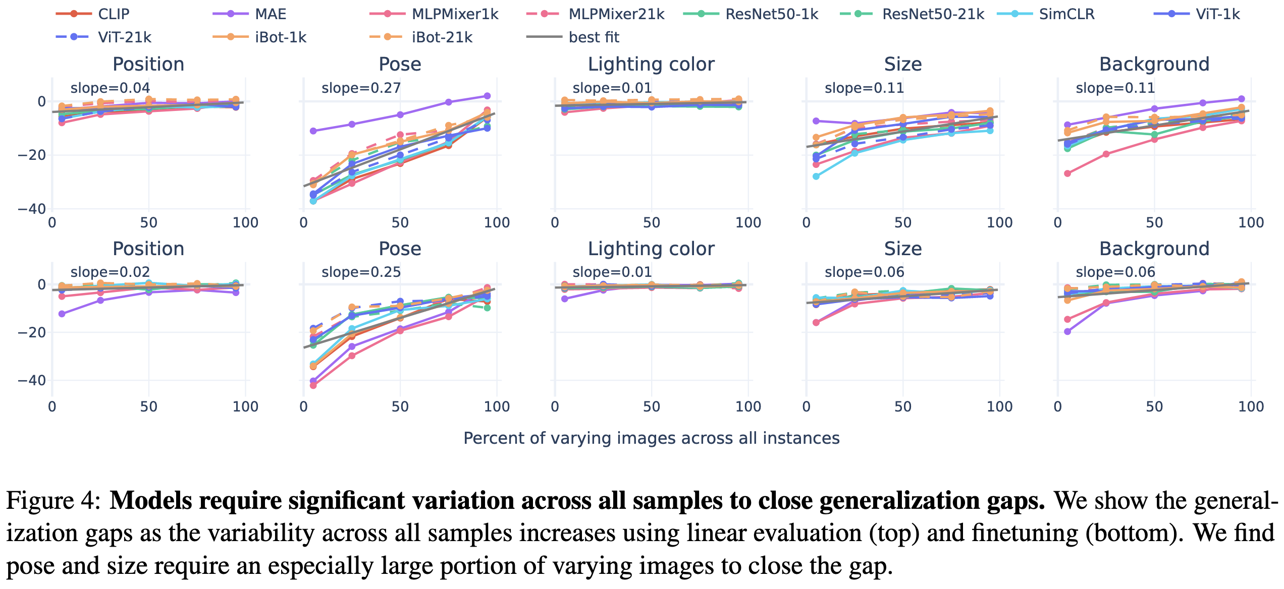
It takes a lot of variation across the training set for the model to learn an invariance.
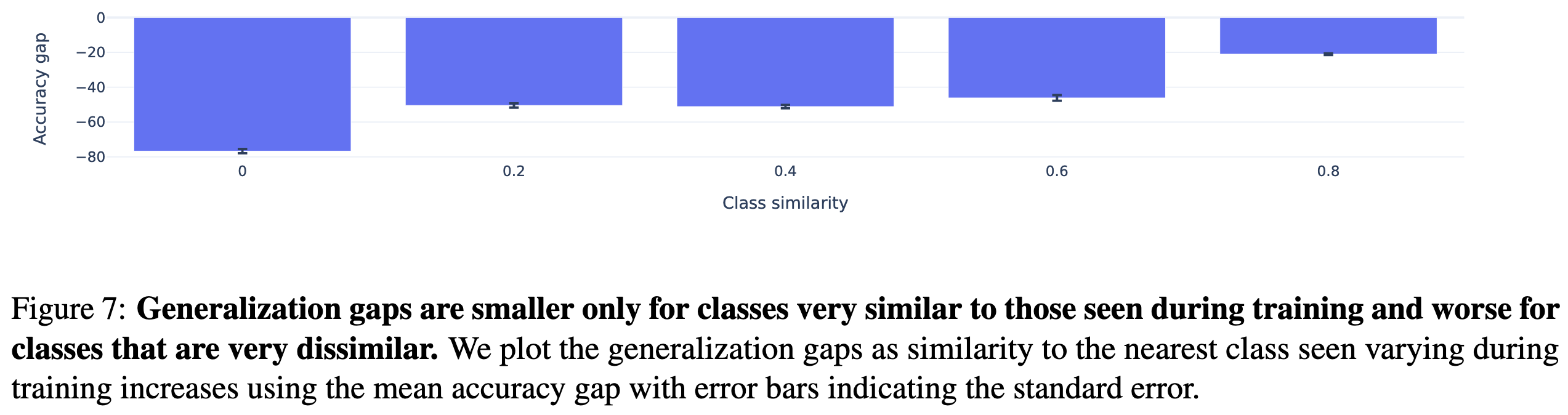
Sadly, consistent with previous work, they find that invariances tend not to transfer across classes. Although there is a nice relationship between how similar the classes are and how much invariance transfers.
On the bright side, varying one factor also yields better invariance to other factors.
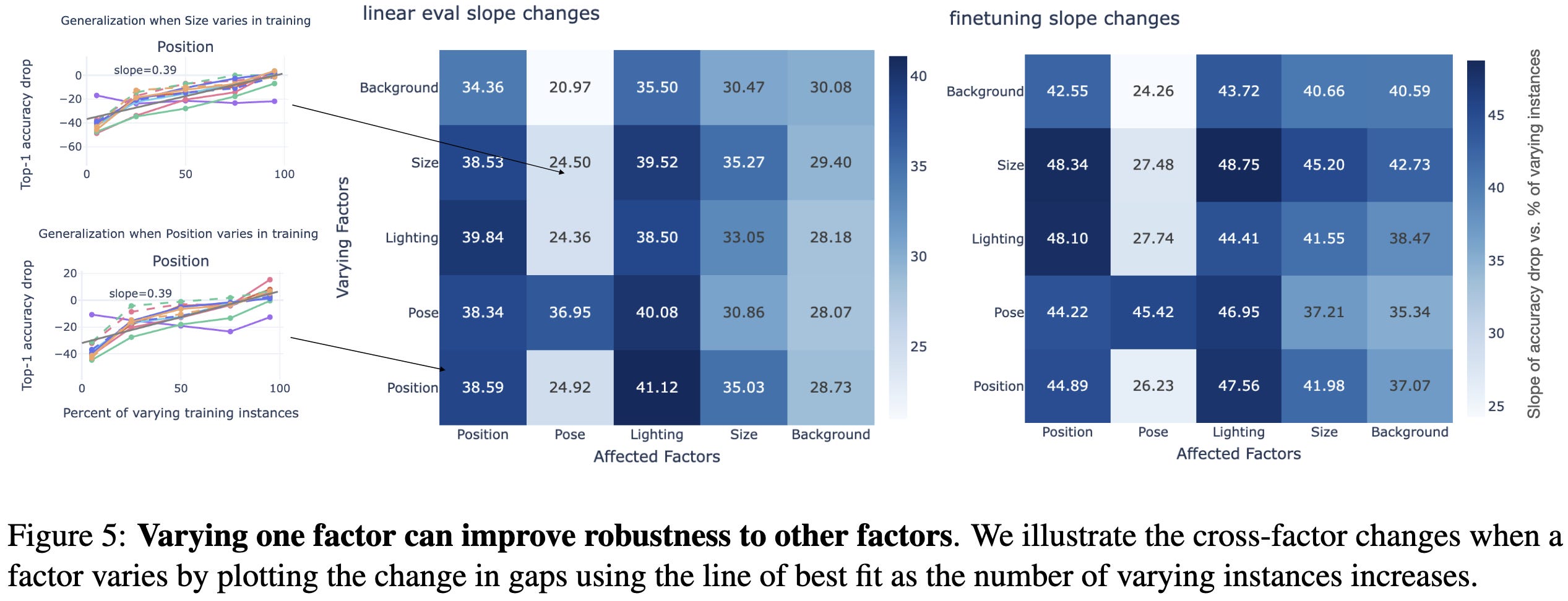
Also, it almost always works to just add all the types of variation to your training set (most bars go to the right, not left, below).
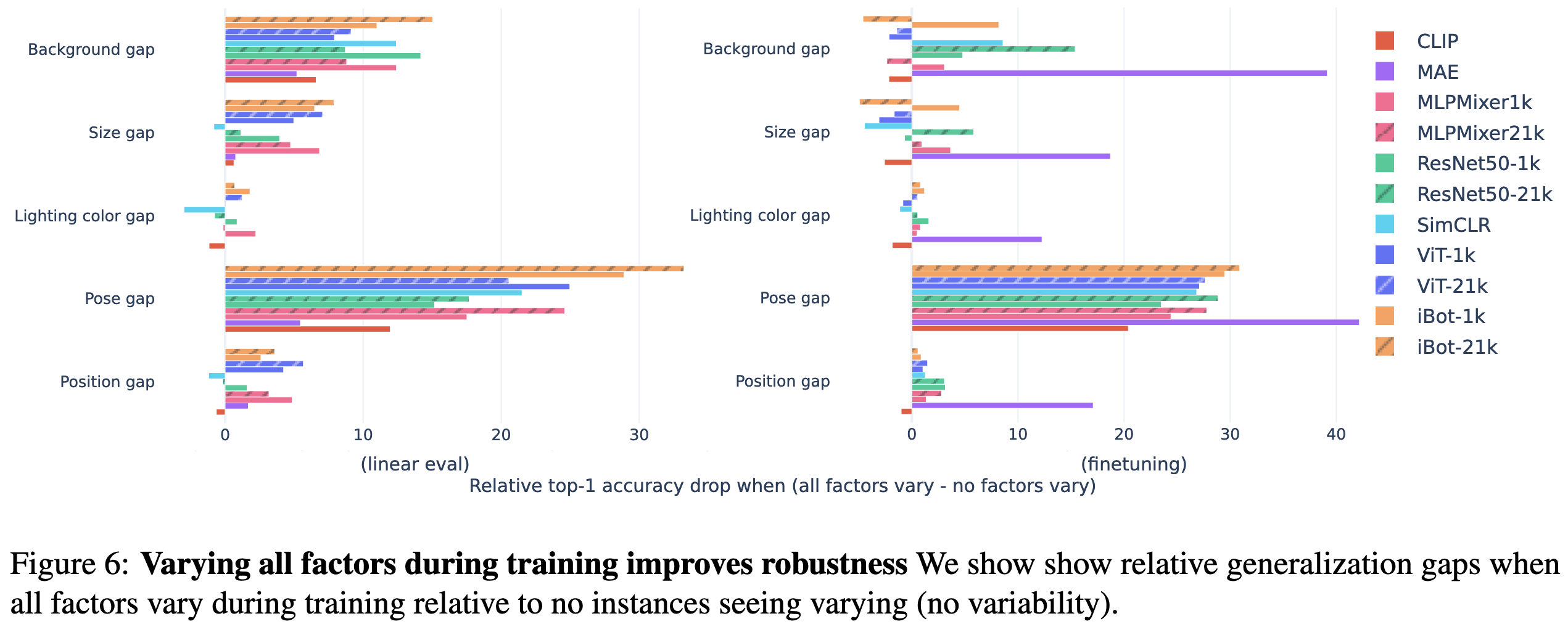
I got excited about playing with their dataset, but it doesn’t look like their code or dataset are available. Still, it’s a thorough science-of-deep-learning paper and cool example of synthetic vision dataset generation.
Class Based Thresholding in Early Exit Semantic Segmentation Networks
Early exit is exactly what it sounds like—aborting the processing of an input partway through the network once you have enough confidence what the label is.
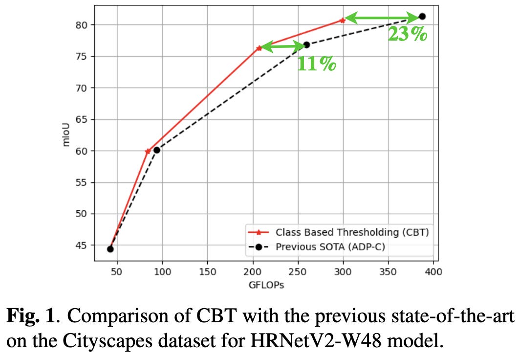
They improve on the most relevant previous method by learning a different confidence threshold for each class. They measure confidence as the gap between the probabilities for the most and second-most probable classes. These probabilities are averaged across all the early-exit layers encountered so far. The confidence thresholds for early exiting depend on the distributions of confidence scores across classes.

Provable Safe Reinforcement Learning with Binary Feedback
Addresses the problem of teaching an RL agent to only take “safe” actions, subject to constraints like only receiving safe vs unsafe labels and not being allowed to take “unsafe” actions even during training.
First of all, I like that they’re thinking through their design requirements rather than jumping straight to making some “standard” metric go up:
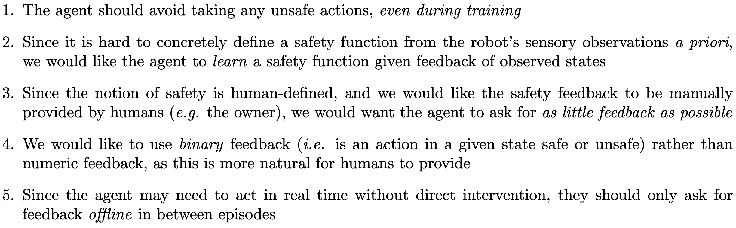
Similarly, they describe their assumptions in detail. One that stands out is that we’ve correctly specified the hypothesis class of the function that maps (state, action) tuples to binary safety labels.

Their algorithm uses any black-box RL algorithm as an input, along with an optional dataset of (state, action, safety) tuples and various hyperparameters.
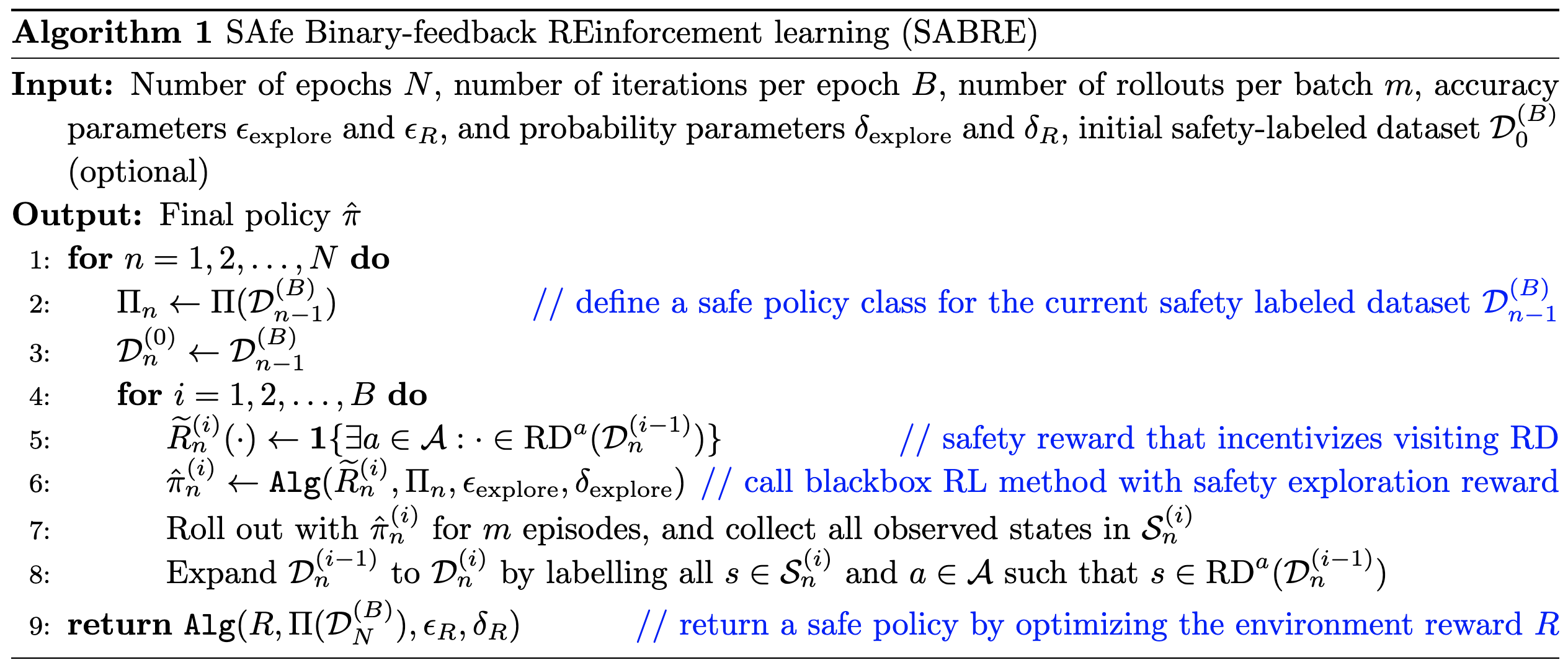
The basic logic is that:
One can provably learn the safety function. This is just PAC learning, made possible by our hypothesis class assumptions.
Given this probabilistic oracle for whether a (state, action) pair is safe, we can refrain from taking maybe-unsafe actions and be smart about when we ask humans for a new label.
You’ll need to stare at the math for a while to really grok it, but this strikes me as really cool. I think of deep learning in general, and RL in particular, as nearly impossible to prove useful guarantees about. Progress on proving safety properties of RL makes me think that tackling AI safety at the RL level is less of a lost cause.
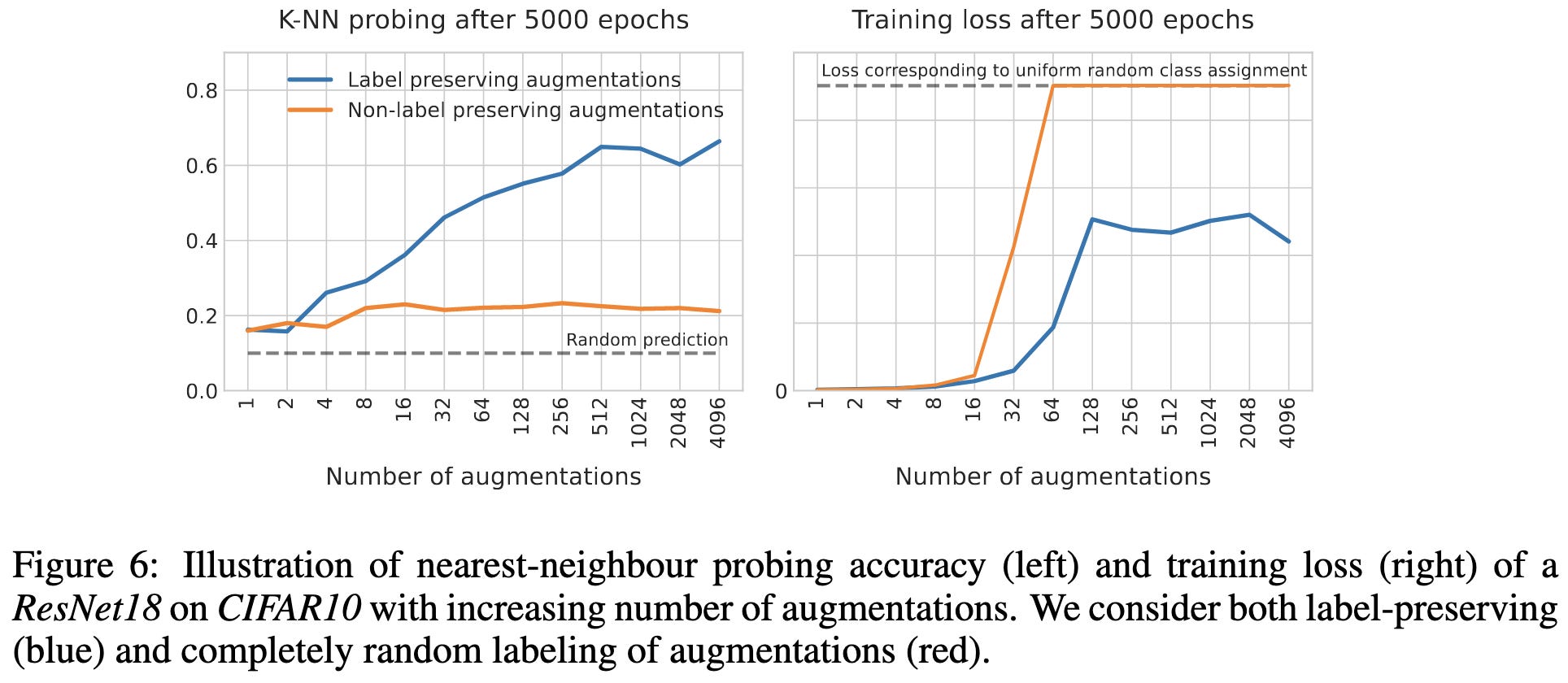
The Curious Case of Benign Memorization
If you train a deep classifier using random labels, all but the last fewer layers end up with useful representations. In fact, the KNN-probe accuracy goes up as you get deeper in the network, until plummeting at the last couple layers.

They argue that a lot of this stems from using label-preserving data augmentations. Intuitively, mapping raw pixels to labels takes more capacity than mapping compact features to labels—even when the labels are random.
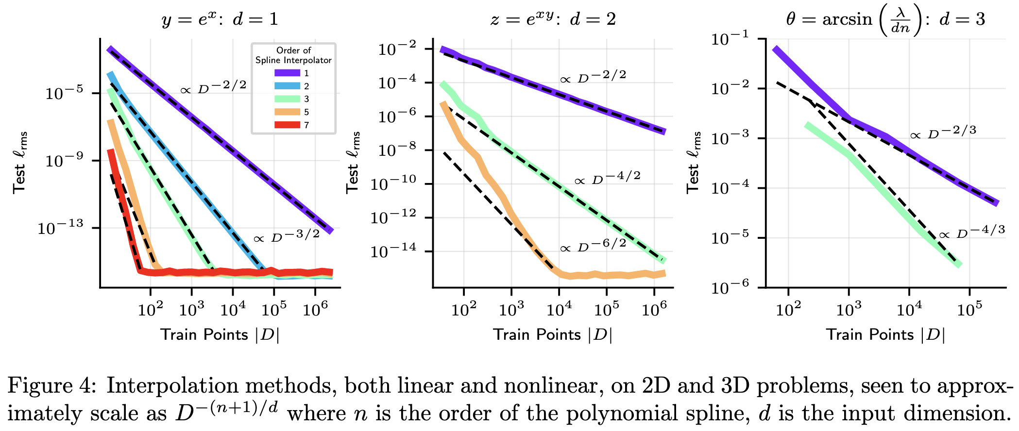
Precision Machine Learning
Let’s say you want to fit a function to your dataset with really low training error. Like, ten-leading-zeros low. Turns out normal training practices won’t get you there.

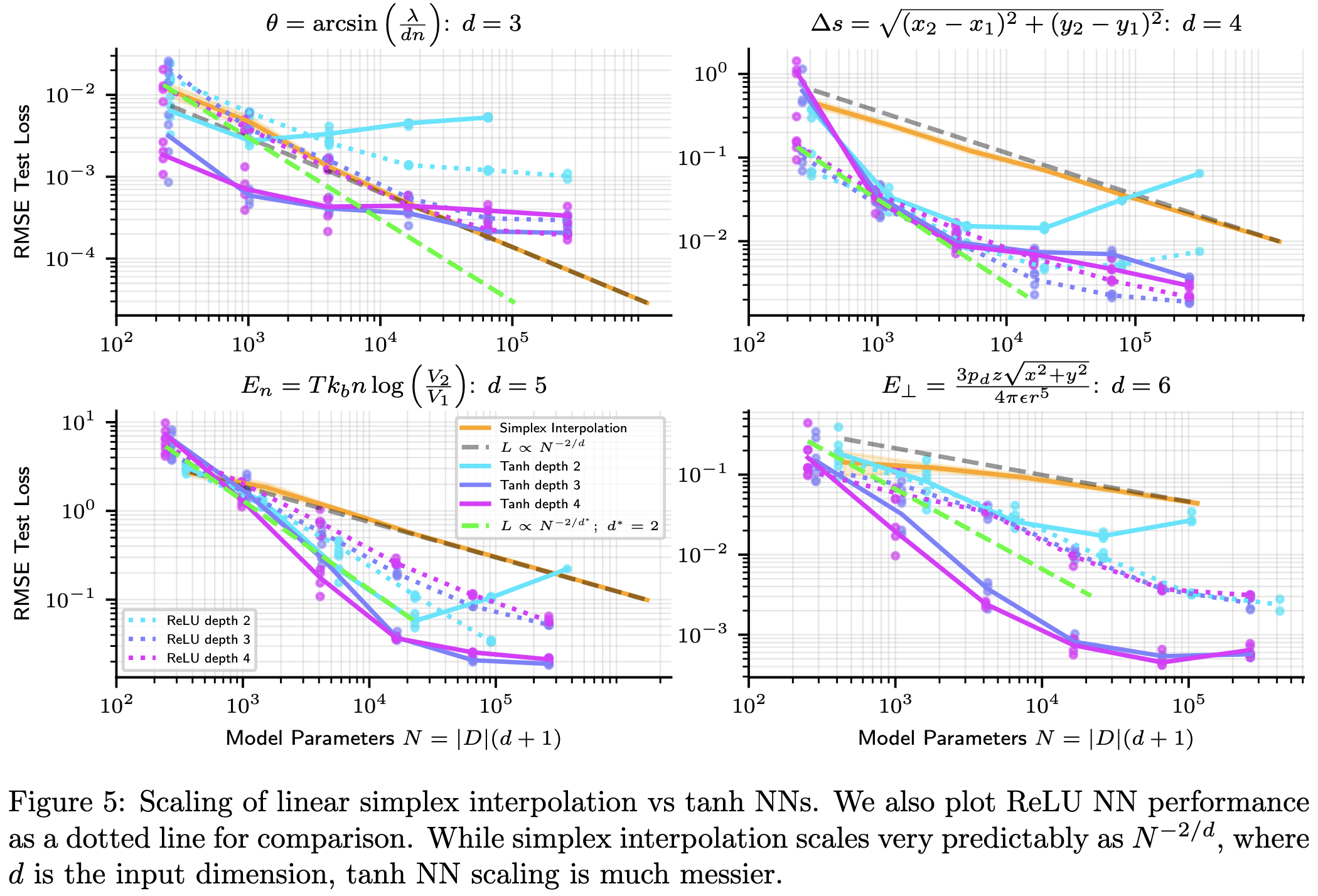
First of all, if you have this problem, they find that you probably shouldn’t use a neural net—unless the points you’re trying to fit are high dimensional.
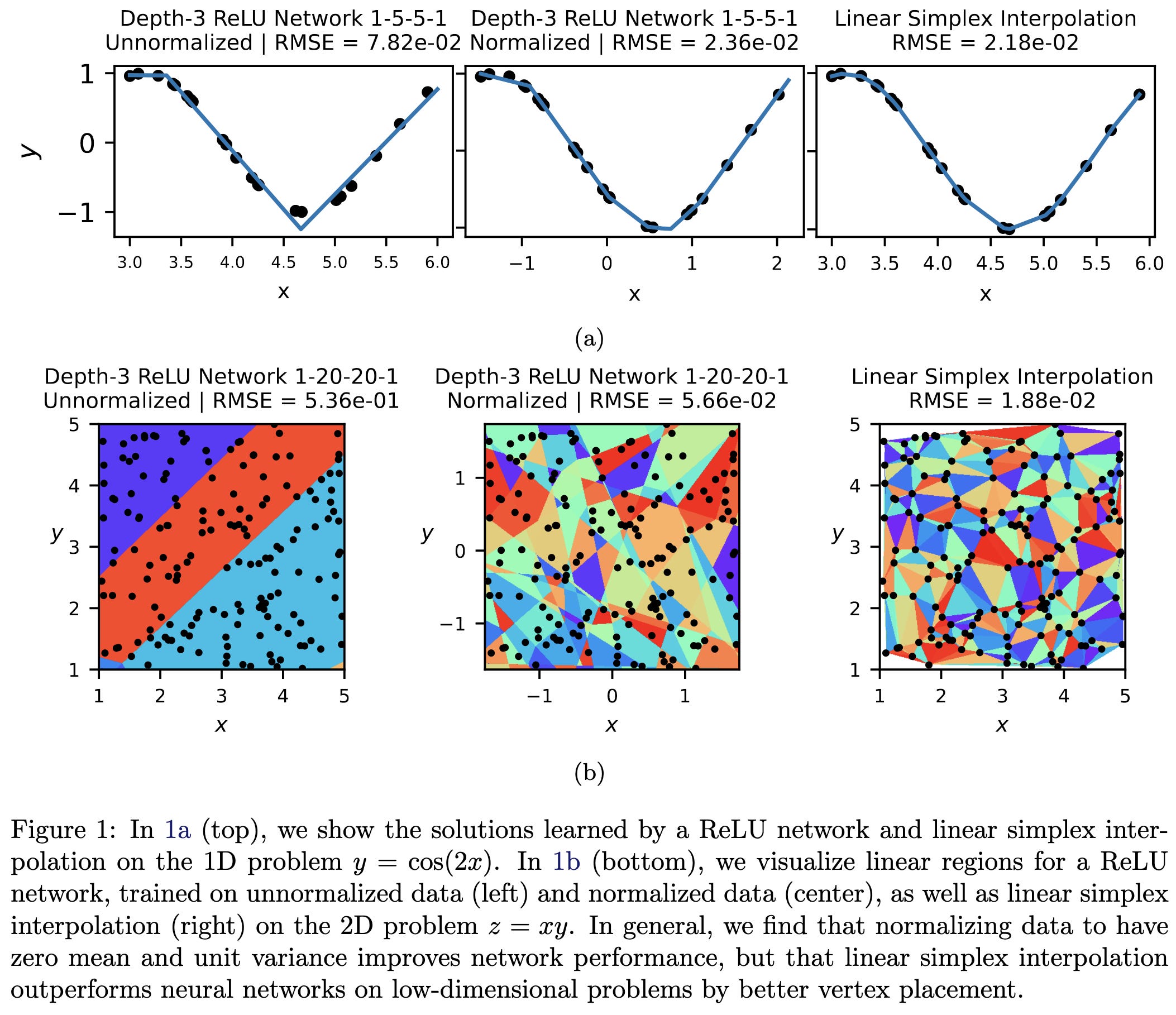
But if your points are high dimensional, neural networks can scale better with both dimensionality and parameter count than alternatives.
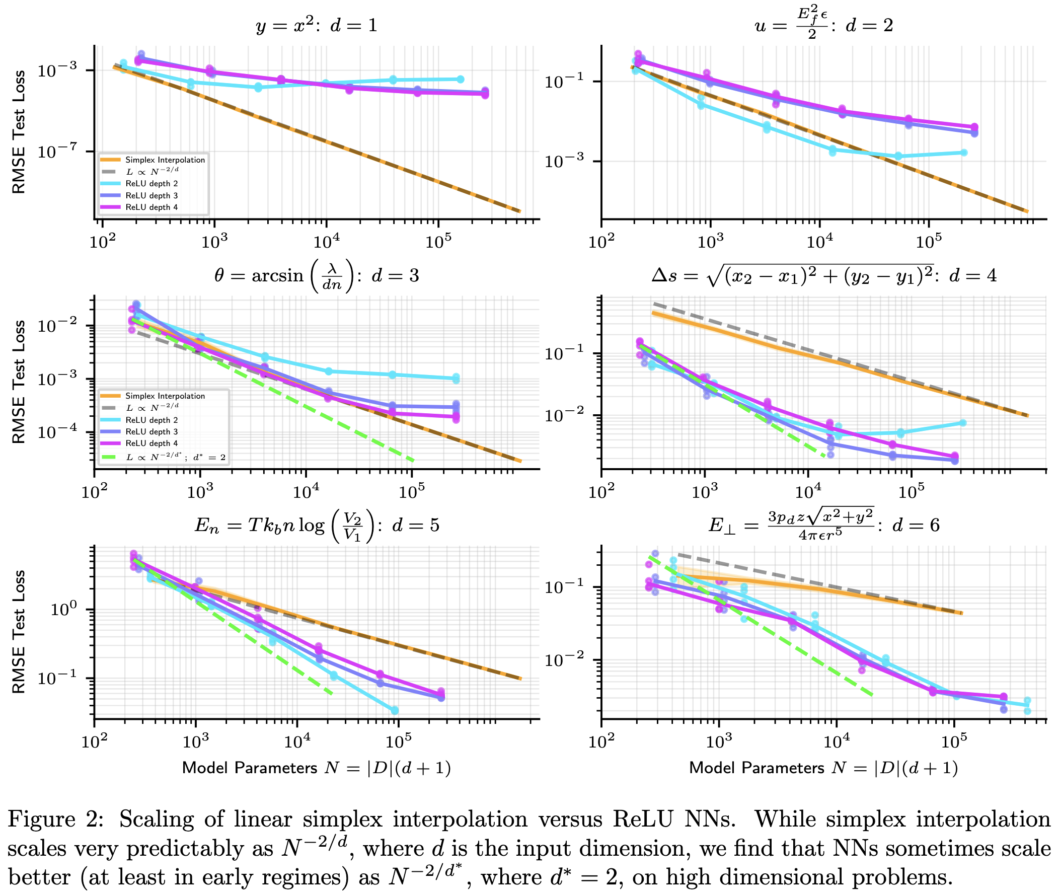
Although sometimes the neural nets are hit-or-miss rather than better.
Side note: they found clear power law scaling for polynomial spline functions, at least until saturating at the numerical limits. Recall that a power law is linear on a log-log scale.
But back to neural nets. With conventional training practices, neural nets can’t fit functions with much precision even when, mathematically, the network is perfectly capable of it.
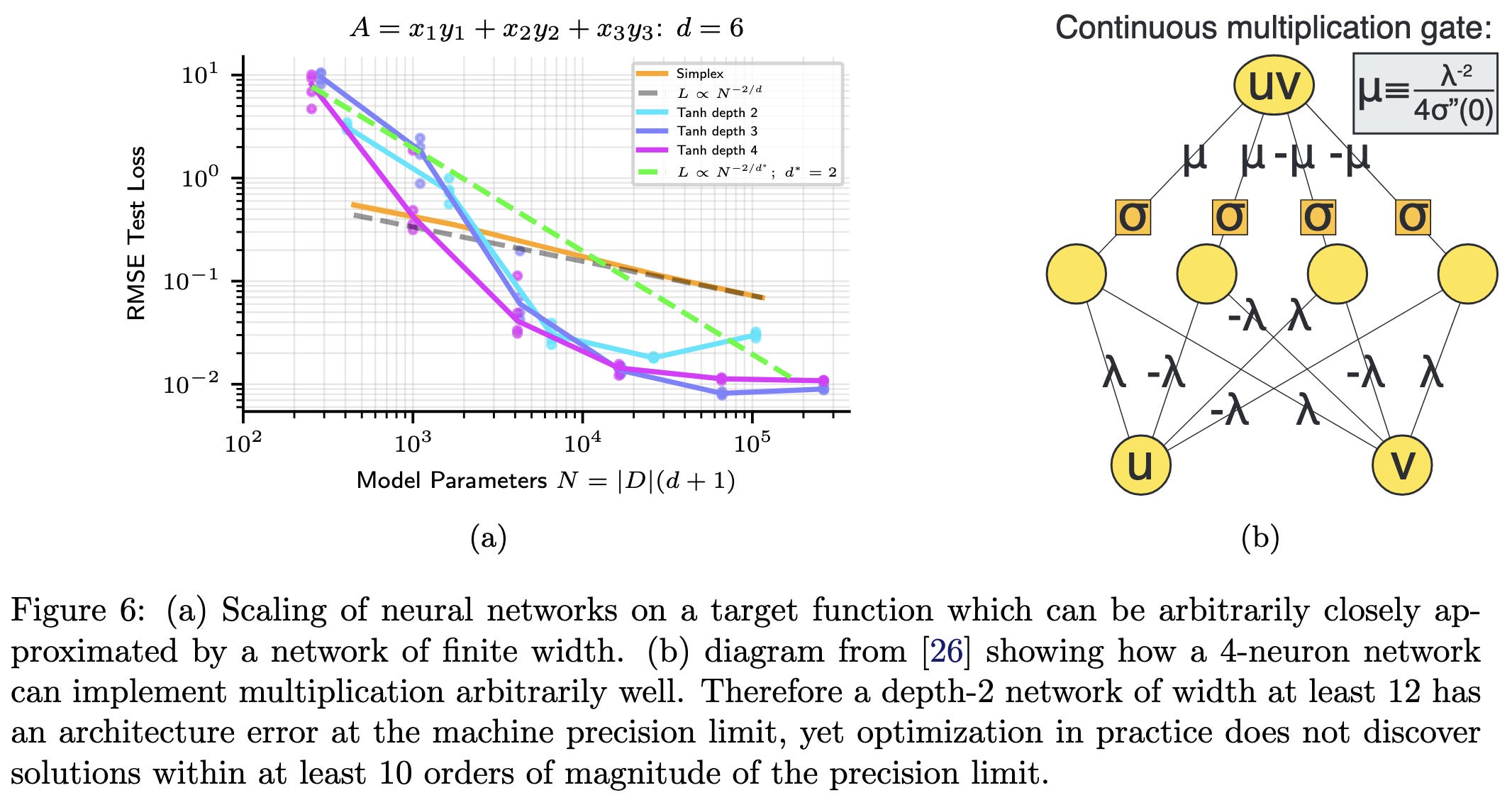
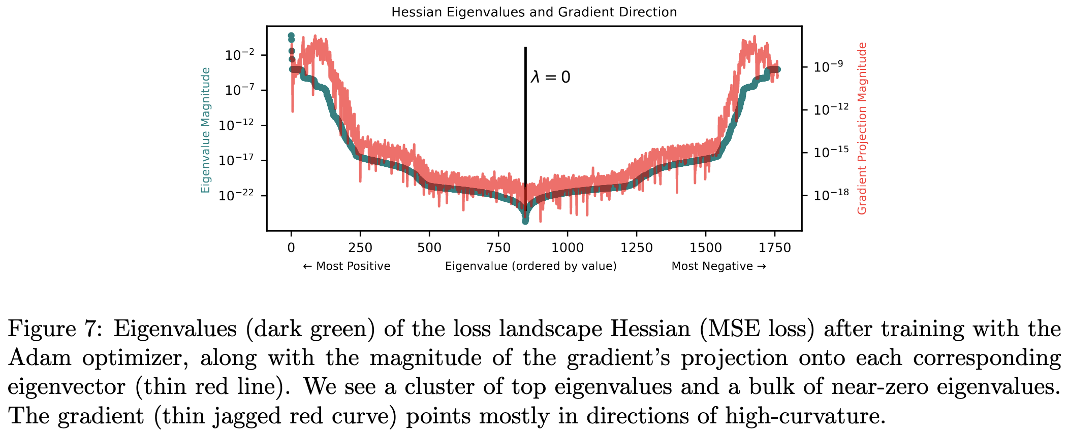
This seems to be because the gradients are dominated by directions with high curvature. So the model just oscillates within a valley rather than moving in the ideal direction.
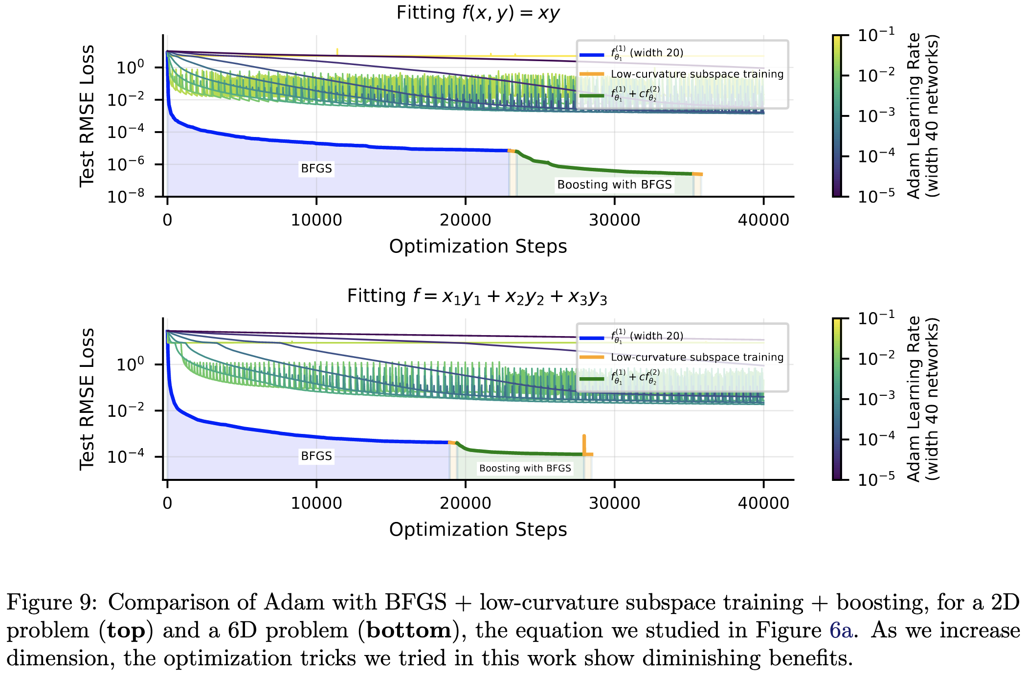
Even with small learning rates, this oscillation causes Adam to hit a precision wall. Using BFGS instead, ideally with boosting, lets you get lower. It can also help to zero out the component of the gradient along all directions with curvature above some threshold.
While they’re largely trying to solve a particular problem, I found this super interesting as a science-of-deep-learning paper. I feel like we all just see our train loss go to some number close to zero and don’t really ask any questions. It’s surprising that we’re sometimes hitting limits 10 orders of magnitude sooner than the numerical limits. Makes me wonder if projecting gradients onto low-curvature directions is just a good idea in general.
It’s also cool that polynomial splines have power law scaling. Are neural net scaling laws just a special case of some more general phenomenon?
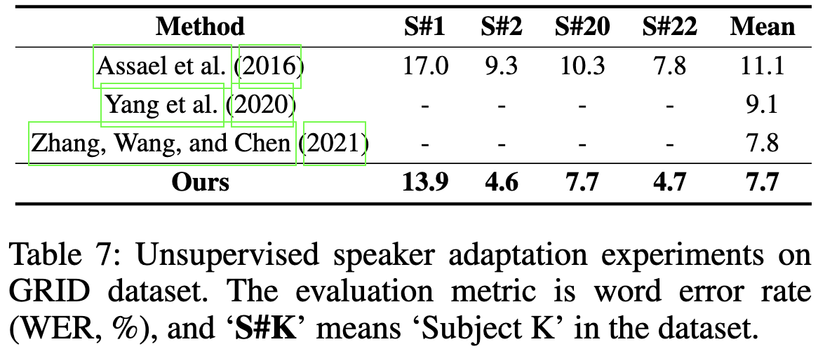
Meta Input: How to Leverage Off-the-Shelf Deep Neural Networks
Rather than apply your model to the test-time input directly, first transform your input to look more like the training data.
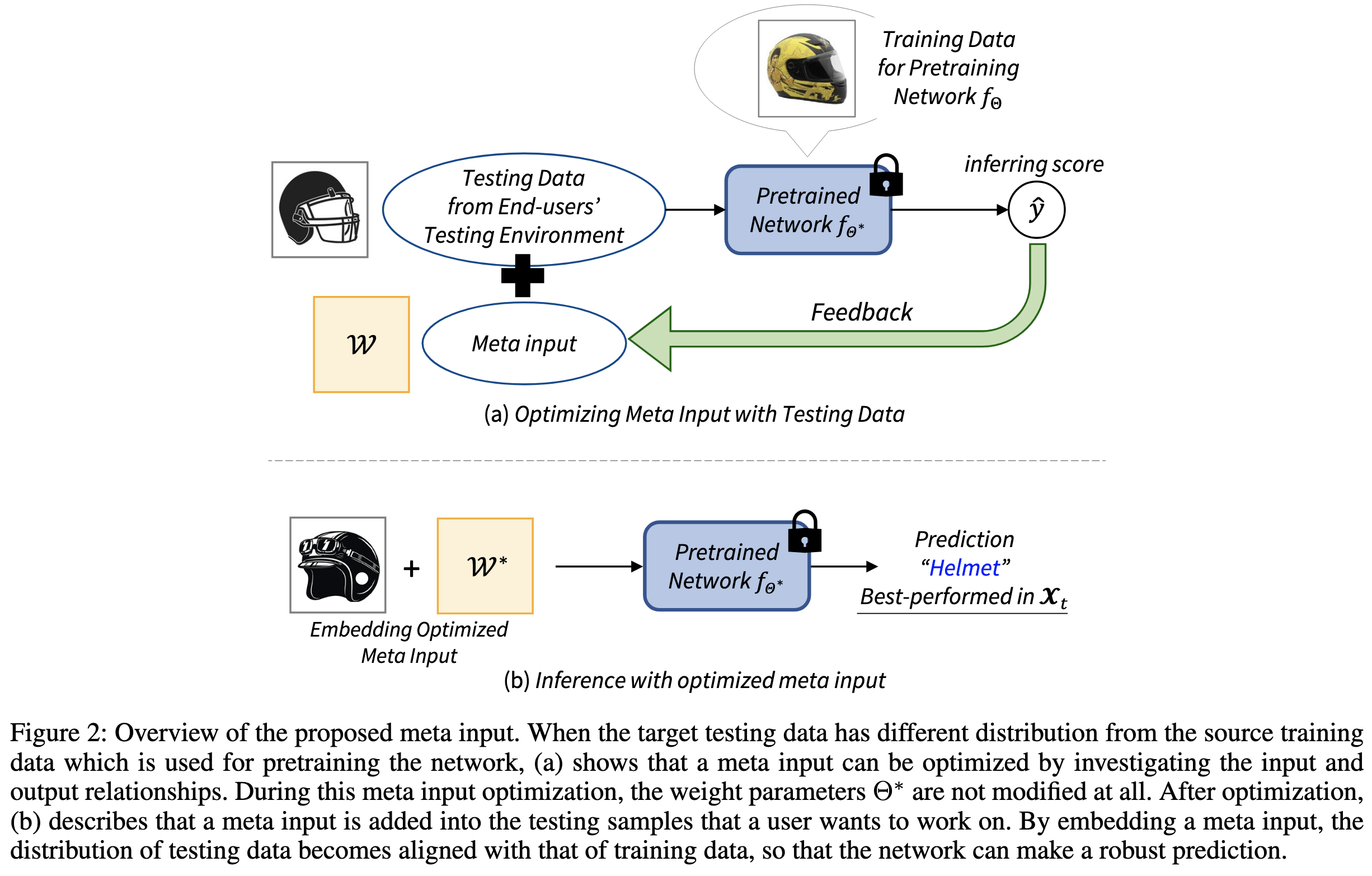
Seems to help with OOD generalization on various problems.


More evidence that there’s a simplicity vs accuracy tradeoff in model serving—i.e., with fancy adaption schemes, we can lift test-time accuracy.
Are we really making much progress in unsupervised graph outlier detection? Revisiting the problem with new insight and superior method
When using the standard noising practices for constructing graph outlier detection benchmarks, simple baselines are often near perfect. They analyze this problem both in theory and practice, and propose a method that beats existing methods based on their insights.
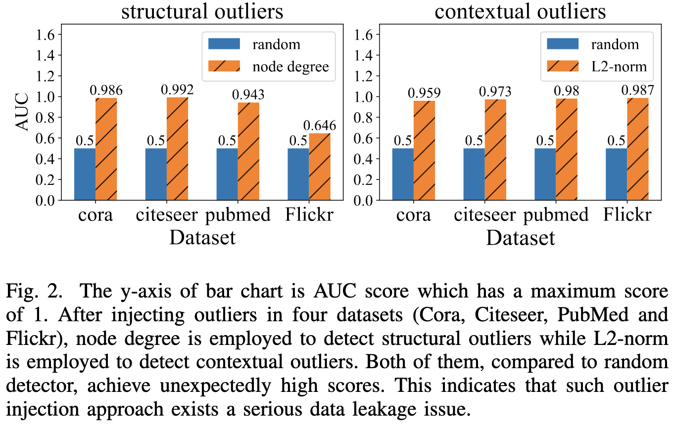
Another entry for my big list of (usually discouraging) ML meta-analyses.
K-SAM: Sharpness-Aware Minimization at the Speed of SGD
They apply selective backprop to the SAM perturbation. I.e., they forward prop the whole batch, but compute the gradient using only the samples with highest losses.

As you might expect, skipping most of the backward pass makes it run faster:
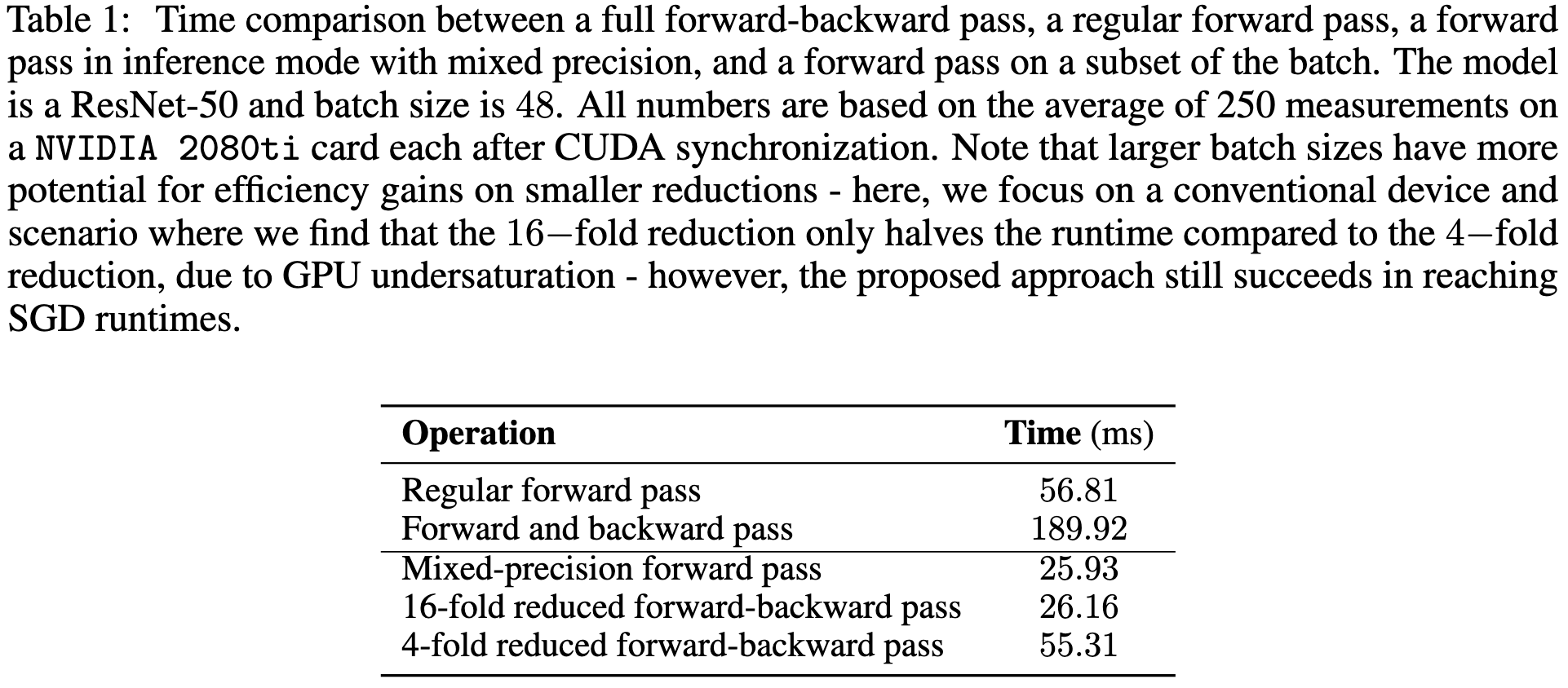
At fixed accuracy, this seems to go a bit faster than SAM—assuming I’m correctly understanding that the right half of this table is actually just two more rows.

The NFNet paper did something similar and found that you could use ~20% of the batch without accuracy loss. Although they seemingly used a random subset of the batch to avoid having to forward prop the whole batch. The present paper finds that uniform sampling like this doesn’t capture the gradient direction as well, although it’s not clear whether that matters.

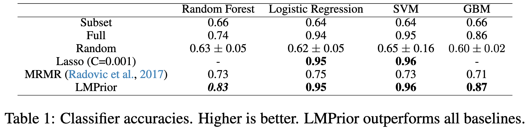
LMPriors: Pre-Trained Language Models as Task-Specific Priors
Describe your task as a prompt with a few in-context examples, and then use the GPT-3 API to get probabilistic estimates of possible outputs. You can then treat these probabilities as priors to combine with any other probabilistic estimator.
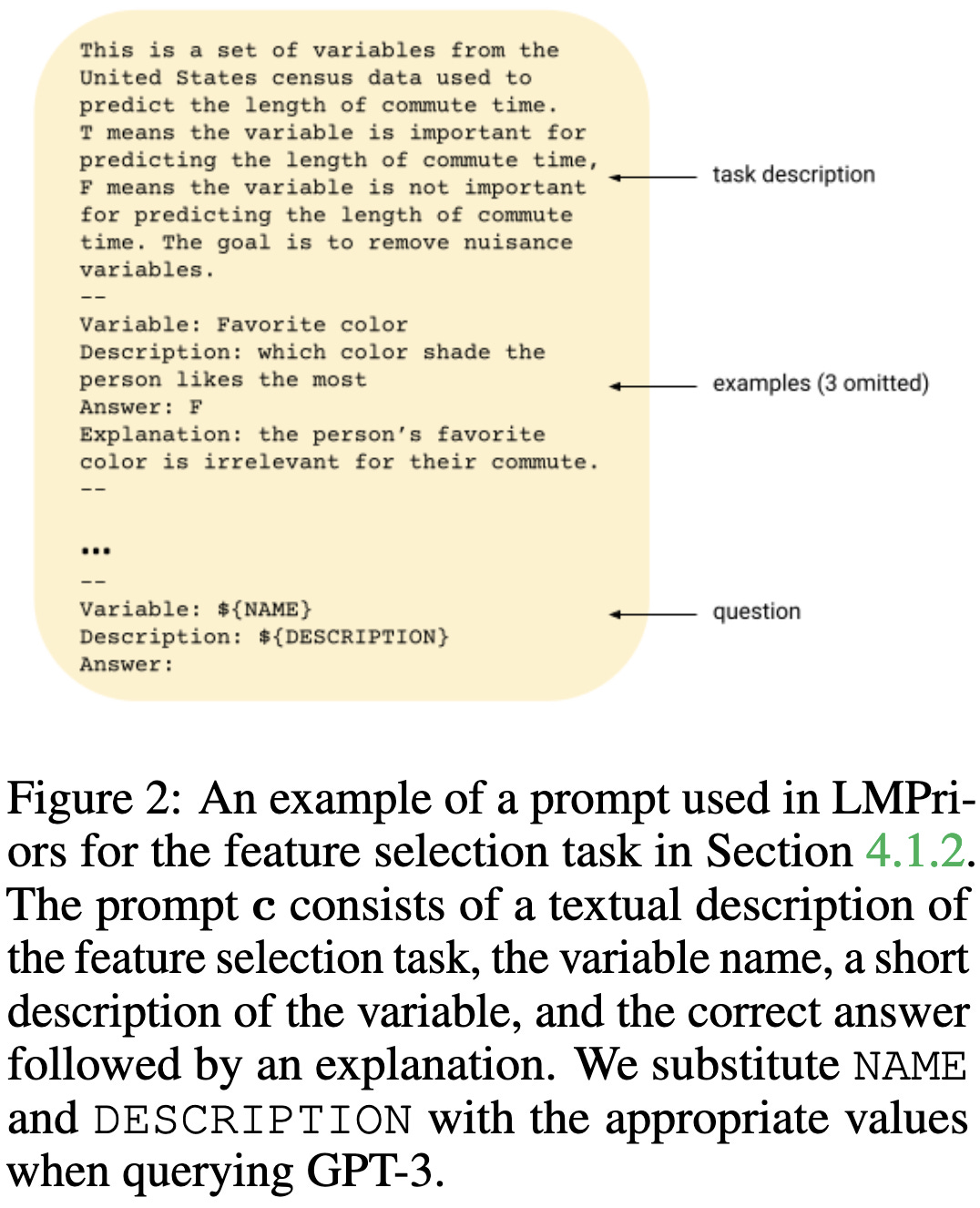
Adding this prior seems to improve classifiers on various tasks.
I see this paper less as “here’s an immediate way to make the numbers go up” and more as “hey, here’s a promising direction for completely changing how we practice machine learning.”
If you look at how people incorporate prior knowledge right now, it’s mostly feature engineering. This is at best an indirect and limited way of capturing knowledge (e.g., we know a ton about biology, but how do you bake that into your clinical risk model?). If we could instead just write up everything we know in natural language, that could be a big win.
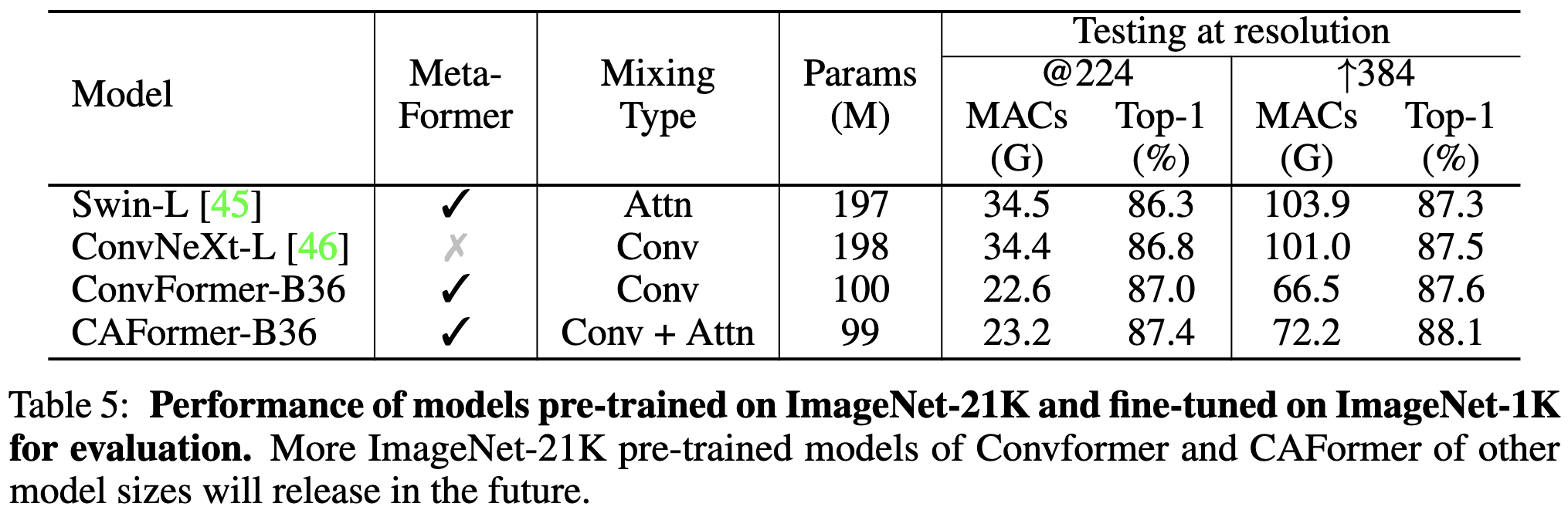
MetaFormer Baselines for Vision
How much of the success of transformers stems from attention vs the overall architecture of the transformer—i.e., alternating token mixing and 2-layer MLPs, along with some layernorms and skip connections?
At least for image classification, they find that it’s almost all about the overall architecture. E.g., you can use any old token mixing scheme (including not at all and mixing with a random matrix) and still get over 80% accuracy on ImageNet.
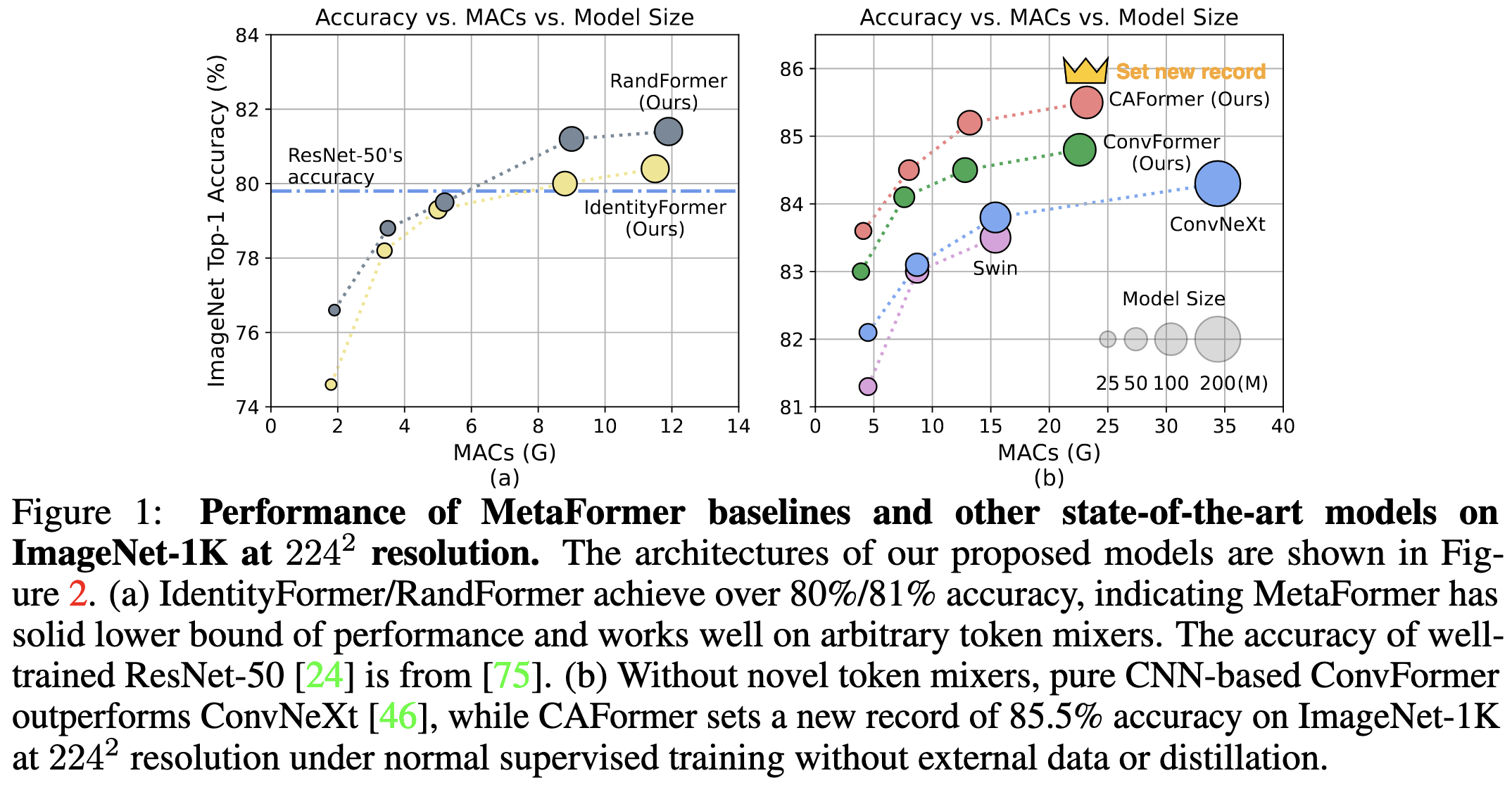
If you want to do even better, you can mix tokens using depthwise separable convolutions (ConvFormer). And if you want to push to a new 224x224 SotA, you can then replace the convs in the top two blocks with self-attention (CAFormer).
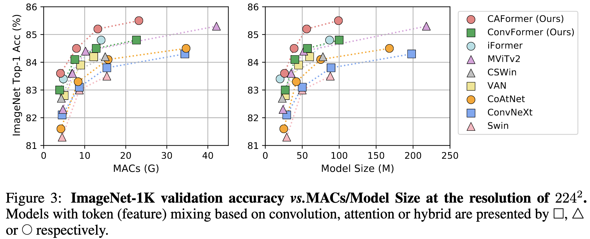
The superiority of ConvFormer and CAFormer also hold for finetuning after pretraining on ImageNet-21k.
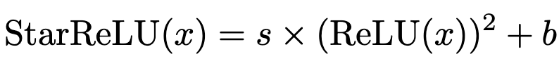
They lift the accuracy further with a different activation function, incorporating a trained scale and bias like Dynamic ReLU.
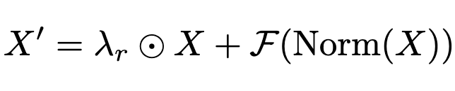
They also incorporate vectors of learnable scale factors for each skip connection (ResScale).
Lastly, they remove all the bias terms in the linear layers. These three extra changes seem to help accuracy.

In practice, it’s not clear that some of these changes are worth it—depthwise convs are super memory-bandwidth bound, as are unfused scale / bias operations. But the core of the paper—showing just how awesome the basic transformer operation is and exploring different token mixing strategies—is great. I’m a big fan of papers asking “why” and not just cargo-cult praising “transformers” or “attention” for being amazing.
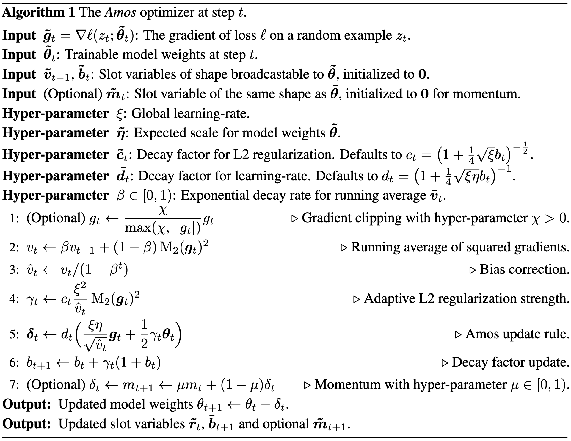
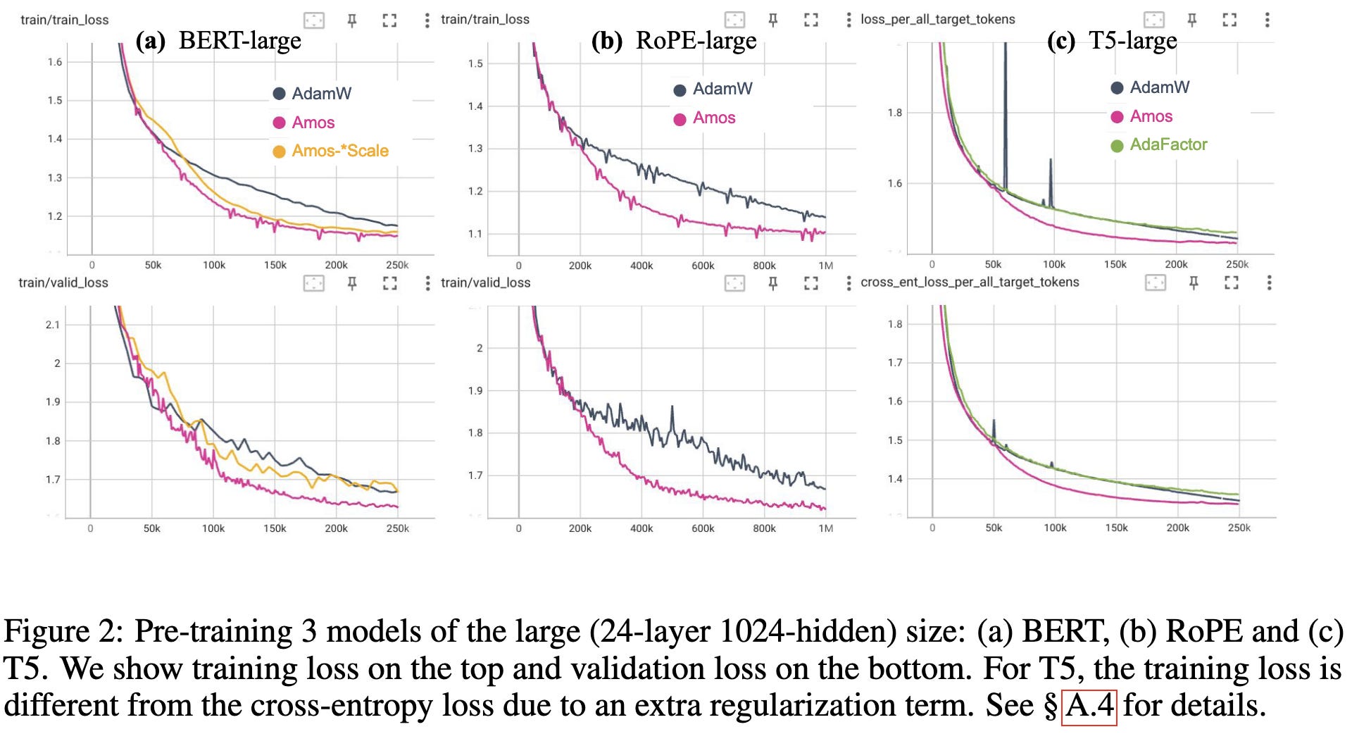
Amos: An Adam-style Optimizer with Adaptive Weight Decay towards Model-Oriented Scale
Another Adam variant claiming to do better. It’s awfully hard to convince me that such an optimizer is actually better given all the lurking variables, but it does have the advantage of only requiring one scalar of state per parameter rather than two. So even if it’s only equal to other Adam variants, there could be a memory win.
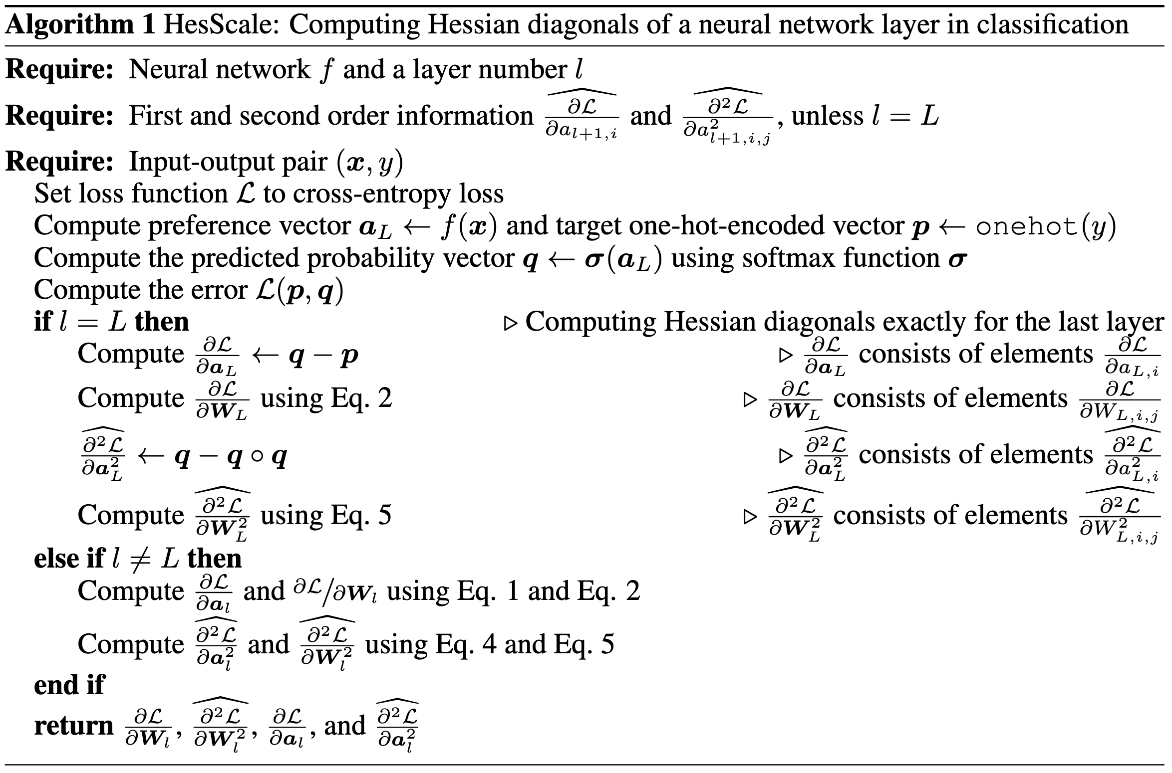
HesScale: Scalable Computation of Hessian Diagonals
They introduce an apparently better method for approximating the local curvature with respect to each of your parameters using the same amount of compute as regular backpropagation (up to a constant factor).
The simplest way to do this is numerically. Just backprop once, perturb the weights, then backprop again. The difference in gradients divided by the perturbation is your diagonal Hessian estimate. But they find that you can do better with local quadratic approximations / backproping curvature info directly (alongside the gradients). And, on top of that, you should use the exact Hessian for the output layer if possible (this is easy for MSE and cross-entropy losses).

Their algorithm yields more accurate Hessian diagonal estimates than alternatives on a toy network.

In terms of speed, it scales pretty well on small models with respect to both the output size and depth (their line is buried in the middle).
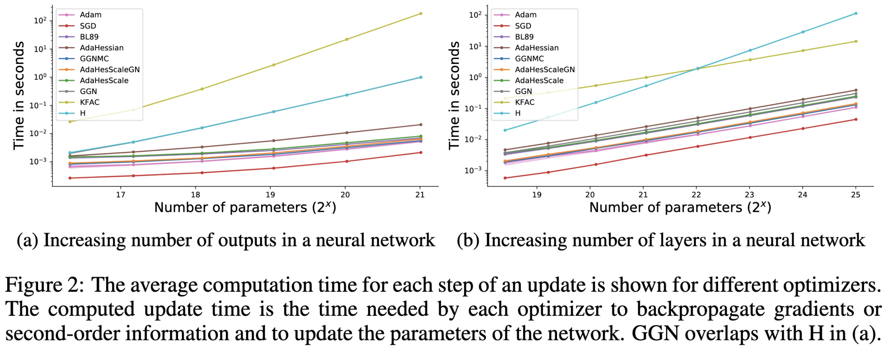
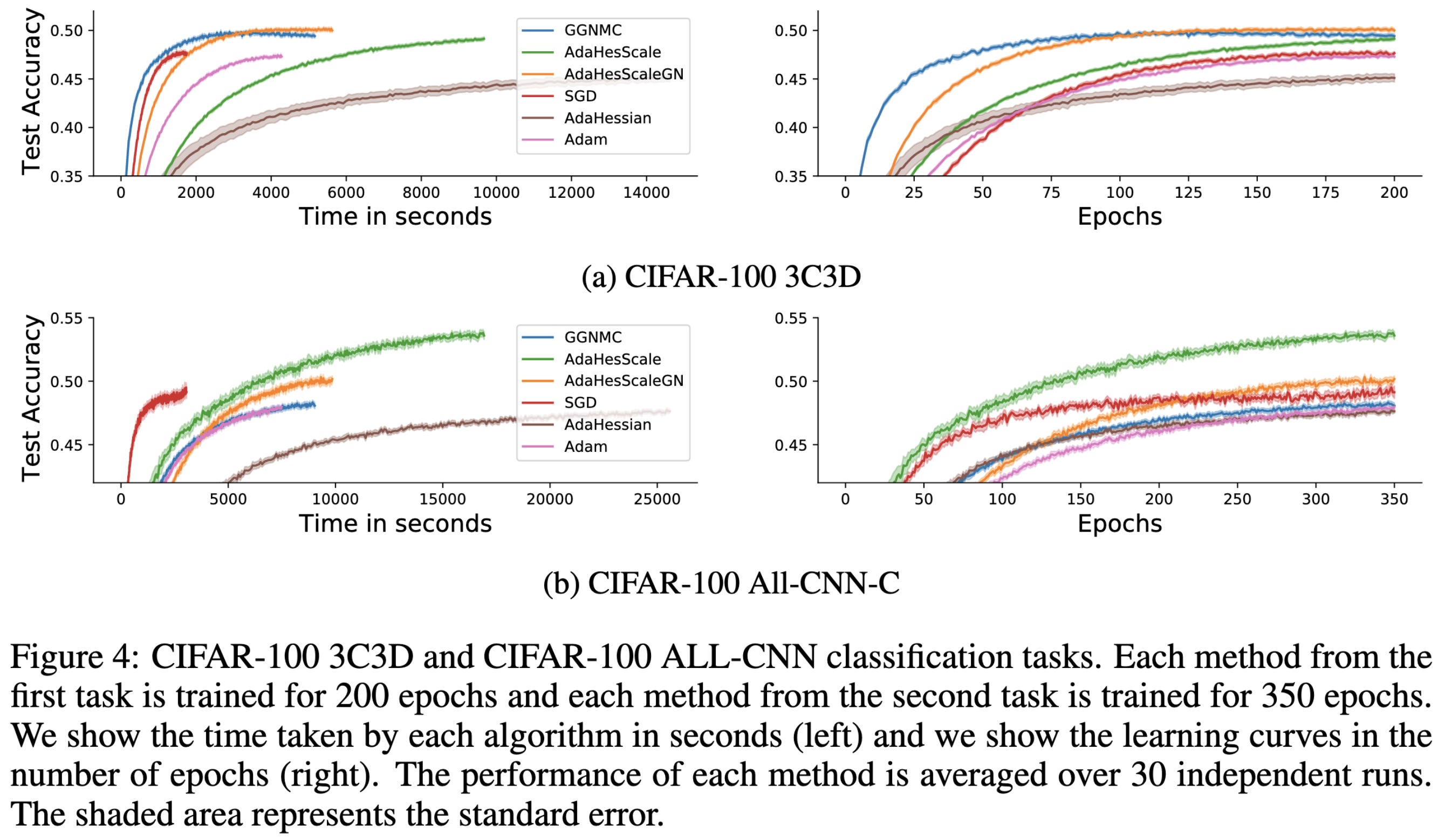
If you use their method to construct a second-order optimizer, you get speed vs accuracy curves that sometimes beat other approaches.
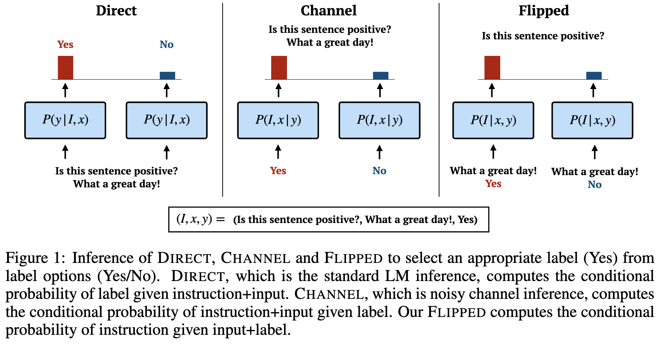
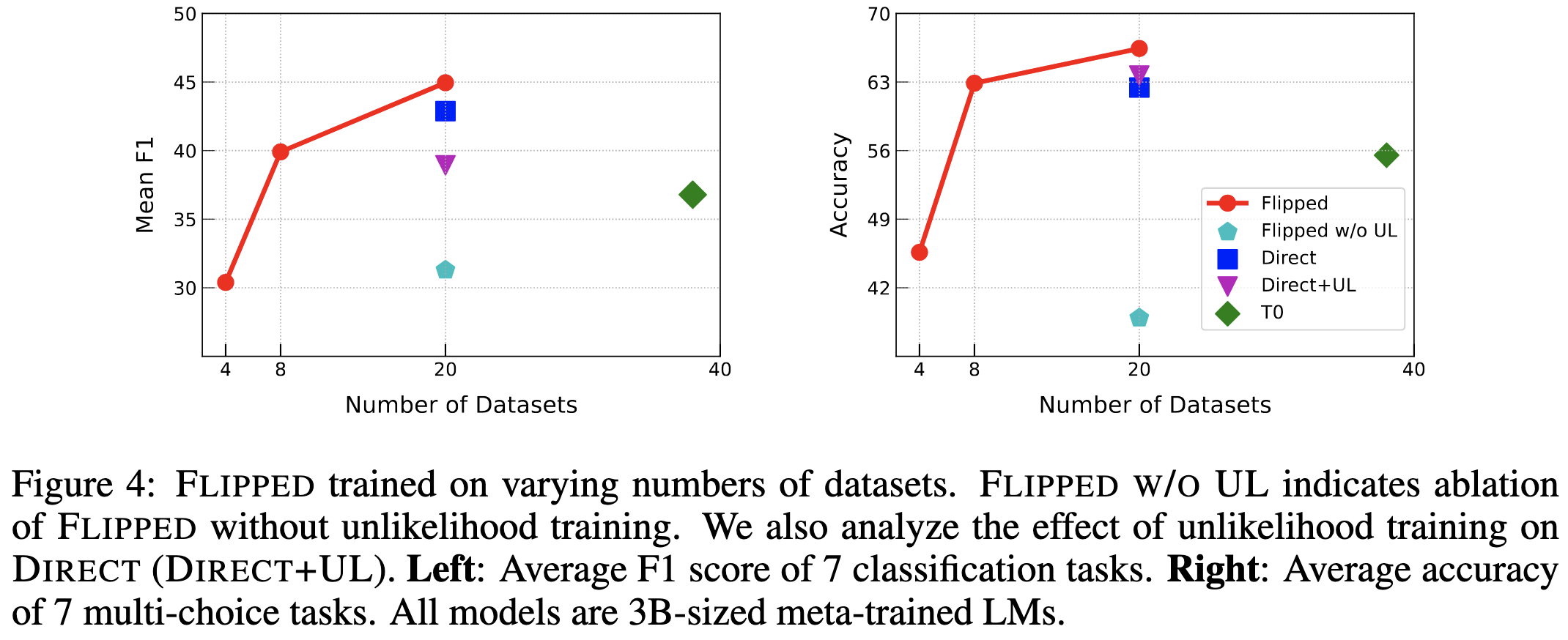
Guess the Instruction! Flipped Learning Makes Language Models Stronger Zero-Shot Learners
Normally we prompt models with an instruction and input and have it output which label is most likely. They propose to instead prompt the model with the input and each possible label and take whichever label is most likely to generate the instruction.
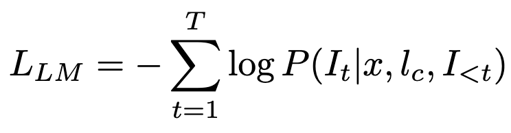
To make this work, they have to finetune the model on instruction generation. Their language modeling loss is below; here l_c denotes the correct label and I_t is a token in the instruction text.
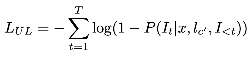
They also add an unlikelihood loss, penalizing association between the incorrect labels and the correct instruction (c’ is an incorrect class).
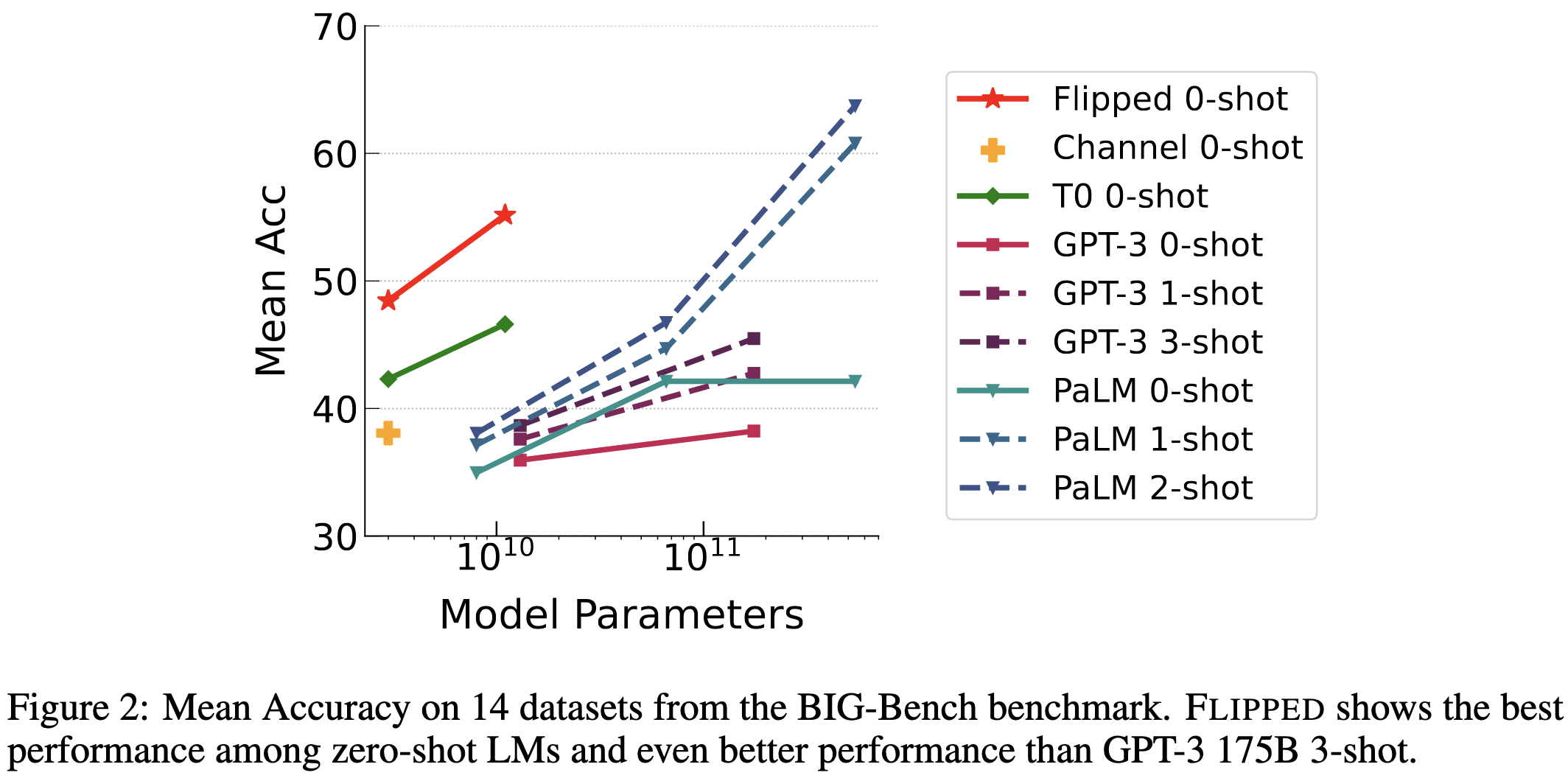
But it apparently works really well in terms of accuracy per parameter.
And their ablations confirm that their design choices probably help (those choices being flipped vs normal T0-style multitask finetuning and having an unlikelihood loss).
My conjecture as to what’s going on here is that they’re just throwing way more compute at the problem per parameter.1 Since they’re only considering classification tasks, the baselines probably make one pass through the input and then only need to generate one token. Whereas here, they’re encoding one copy of the input per possible label and then generating a whole instruction.
We’ll need follow-up work to know for sure what’s going on here though. Either way, these are interesting and promising results.
I also suspect this explains much of the apparent superiority of diffusion models. By applying the decoder dozens or even thousands of times, you screw over your FLOP count but do way better at a fixed parameter count. I don’t follow the literature closely, but have yet to see a FLOP-matched comparison showing diffusion models beating VAEs.