2023-1-8 arXiv roundup: Language models creating their own data, Hinton vs backprop, Practical pruning + quantization for LLMs
This newsletter made possible by MosaicML. Feels like we have some
Massive Language Models Can Be Accurately Pruned in One-Shot
They prune 50% of the weights in huge OPT models with little or no loss of accuracy and no finetuning.
The basic approach here is to go layer-by-layer and iteratively:
Rip out one low-magnitude weight in each row
Update the remaining weights to optimally approximate the original layer (in a least-squares sense, evaluated on a sample of 2^19 tokens).
This is hard because, to compute the least-squares solution, you need the inverse Hessian matrix for the remaining nonzero columns. But every row can have its own sparsity pattern, so a naive solution would take num_rows * num_weights_pruned_per_row giant matrix inversions. This would take hundreds of hours at best at this scale.
To make this iterative pruning + least-squares approach feasible, they introduce a clever greedy algorithm:
What this algorithm does at each layer is the following:
Compute the Hessian for the whole input matrix X. (This is what lets us compute the least-squares solution in closed form.)
For each column:
Remove the contribution to the inverse Hessian from the previous column. This is an n^2 (not n^3 !) rank-1 update.
Pick some elements to prune in this column. This decision looks at blocks of 128 columns at a time, not just one, so that not all columns have to be pruned the same amount.
After pruning, update the remaining values in each row using our new Hessian.
The sense is which this is greedy is that it 1) selects which entries to zero out in a greedy fashion, and 2) never updates the non-pruned weights in earlier columns to account for later pruning.
Another nice feature of their method is that you can easily integrate quantization. The obvious way is to just quantize after pruning, but you can do even better by quantizing the non-pruned values in each column after pruning. This lets us update our remaining weights to account for the quantization noise in addition to the pruning.
The results are impressive. They lose little or no model quality with 50% unstructured pruning, and not much quality with structured pruning. Crucially, the 2:4 sparse model is still much better than the next smaller model, meaning you could probably get an improvement to the latency-accuracy tradeoff in practice.
Even more impressively, you can both quantize and prune without much of an accuracy hit on large models—though this isn’t true with 2:4 sparsity.
Mostly this convinces me that it’s totally doable to use NVIDIA’s 2:4 sparsity acceleration for inference with huge models—and it might be possible for training as well. Sparse / quantized training is much uglier from a software perspective, but would probably preserve the accuracy even better.
The case for 4-bit precision: k-bit Inference Scaling Laws
They find that, to get the best inference RAM vs accuracy tradeoff, you should probably use the largest model you can and 4-bit quantize it. I.e., you’re better off with a 20B parameter 4-bit model than a 10B parameter 8-bit model.
This pattern holds across a variety of model families. Also, 3-bit does surprisingly poorly, even when you quantize the outlier values separately. And 4-bit quantization seems to not need outlier quantization as long as you use group-specific quantization parameters for small enough groups of parameters.
The main subtlety here is that there are zero speed savings reported. This is because they convert each quantized tensor back to f16 before operating on it, so they have extra overhead and never get to use faster low-precision math. With good kernels though, I suspect you could get some speedup for small matrix sizes (which are more likely to be memory bandwidth-bound).
Mostly this makes me wonder how much better we could do throwing real compression algorithms at the problem, rather than just using scalar quantization as a heuristic lossy compressor. For activation and gradient compression, compression usually isn’t worth it from a time vs accuracy perspective. But if our goal is just size vs accuracy, I bet we could go really small.
The Forward-Forward Algorithm: Some Preliminary Investigations
Geoff Hinton tries to replace backprop. The idea here is to assign each layer’s activations a “goodness” and then just update the parameters within a given layer to maximize the goodness for real samples and minimize it for synthetic samples.
The goodness they consider is just the sum of squared activations. This is convenient both because it’s simple and because adding a LayerNorm after each layer makes the next layer’s inputs all look equally “good”—unless that layer succeeds in learning something about the real + synthetic distributions.
The experiments are all on MNIST and CIFAR-10, so the synthetic data is just images from a handcrafted pipeline.
To allow information to flow from higher layers to lower ones, they treat static images as a video (with all frames equal to the image) and allow each layer’s representation to be informed by the next and previous layers’ outputs at the previous timestep.
The results don’t yet demonstrate that this method is likely to be beat backpropagation, but I think it’s really interesting on a direction-setting level.
First, it identifies some ambitious design goals. These include:
Allowing better (pipeline) parallelism than backprop
Allowing an offline “sleep” phase and an online “wake” phase. This could enable training on only positive samples (the “wake” phase) for long stretches of time.
Facilitating analog hardware by avoiding the need to exactly store activations for subsequent gradient computation
Enabling “mortal computation.” This means that, instead of paying all the time + energy costs of getting programs to run identically across hardware, we just build hardware and have our learning procedure deal with the machine-specific variation. I.e., what happens in living organisms.
This last one is super interesting and not something I’ve heard anyone mention before. I could imagine large wins if we could set our chips’ clock rates based on, say, 90th percentile switching latency rather than the 99.9999th percentile (or whatever huge safety margin is needed to make digital logic reliable). Similarly, fabs could get ~100% yield if faults in the chips all got magically handled at the software level.
On the other hand, not having software run the same on different devices would be a nightmare from a debugging and deployment perspective. Though maybe the program is the same and you just get tiny accuracy variations, which few-shot learning deals with after just a few trials.
Lastly, I just want to give props to Geoff Hinton for writing papers like this. In the history of science, usually what happens is that the famous researchers make some great discovery when they’re young and then spend the rest of their careers being sticks in the mud and arguing that their theory is right and all the new stuff is wrong. But in machine learning, we have Hinton (and others) basically saying, “All that stuff I helped pioneer still isn’t good enough and we need to think outside the box to do better.”
Plus this paper has some great perspective on different techniques, their shortcomings, and the relationships between them, delivered in a way that only someone with decades of experience could pull off.
So I’m not sold on the exact method, but I still feel like this is an exceptionally interesting paper.
GPT Takes the Bar Exam
They administered a Bar Exam (needed to become a lawyer in the U.S.) to OpenAI’s text-davinci-003. It’s not as good as the average test taker and is only on track to get a passing grade in three of the seven categories.
What’s interesting is how much better ChatGPT is. In less than the time it took for the authors to execute this project and write this paper, GPT variants went from failing to passing the bar exam.


And while it’s at it, ChatGPT apparently passes the equivalent exam for medical doctors.


As with all results, there are a bunch of questions here (could the practice exams they used be too similar to the training data? How much does omitting questions with images matter? etc). But the fact that the rate of progress is faster than the publication cycle is pretty striking.
Cramming: Training a Language Model on a Single GPU in One Day
They run a ton of experiments to figure out the best way to train a BERT-like model in one GPU-day. This is less a paper with one central idea and more a paper with a ton of empirical observations.
First, consistent with previous work, they find that the size of the model matters a lot, but different transformer variants all do about the same.
To exploit this observation, they tweak their initial BERT in ways that preserve the parameter count while decreasing the runtime. Changes that helped:
Removing the biases from the {Q, K, V} projections in the attention layers
Removing the biases from the rest of the linear layers
Adding GLU to the GELUs in the FFNs (and not adding more parameters to compensate for the reduced hidden dimensionality)
Scaled sinusoidal positional embeddings (vs learned or unscaled embeddings)
Using Pre-LayerNorm rather than Post-LayerNorm. Though it doesn’t help on its own—only indirectly by making training stable / enabling larger learning rates.
Removing the nonlinearity in the (MLM?) head to save time at no accuracy loss
Sparse token prediction (like RoBERTa)
Disabling dropout during pretraining (but not finetuning)
Changes that didn’t help:
Reducing the attention head count (faster pretraining but worse finetuning quality)
Attention variants including FLASH and Fourier attention (unsurprising given that their sequence length is 128)
RoPE (higher accuracy, but not worth the time—contrary to GPT-Neo-X findings)
Using activations other than GELU in the FFNs
In addition to altering the model, they also mess with the training recipe. The only thing that helped was ramping up the batch size linearly throughout training (via gradient accumulation). What didn’t help included:
Automatic / adaptive batch size rules
Messing with the Adam hparams or using second-order optimizers
Using a masking rate higher than 15%
Replacing 10% of the masked tokens with random tokens and leaving 10% unchanged like in the original BERT paper
Using mean-squared error or L1 loss for the mask prediction
They do find that using one-cycle-like learning rate schedules helps. But in my experience you need to control both the area under the learning rate curve and the final learning rate for this to be an apples-to-apples comparison. Also you usually need to standardize the warmup. So it’s not clear IMO where it’s the schedule per se that helps or these other factors.
Lastly, they assess a variety of changes to their data pipeline. What worked includes:
Using The Pile rather than C4
Removing sequences that had too many tokens relative to their length (a measure of compressibility / how typical the sequence is)
Sorting sequences by the average unigram probabilities of their tokens, with more typical sequences coming first. This seems to work especially well if you also ramp up the dataset size so that the most atypical sequences are never reached.
What didn’t help is:
Using a large vocabulary size also helps, at least up to a certain point.
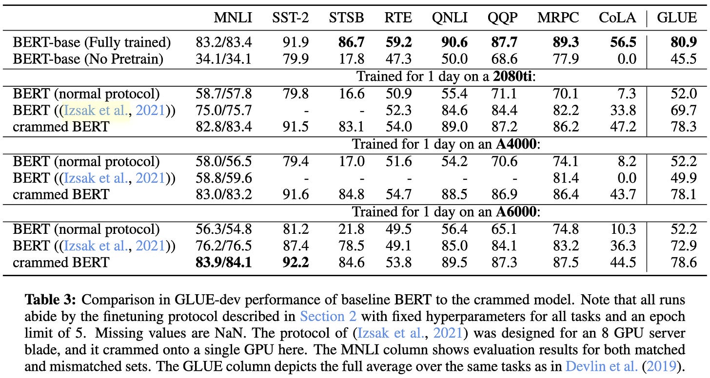
Combining all of their positive results together, they get much better GLUE results after 24 hours of training than a vanilla BERT training setup.
I found this paper exceptionally useful. If you’re trying to squeeze as much as you can out of a BERT model (or maybe even a transformer more generally) I would definitely recommend giving this paper a careful read.
Tutel: Adaptive Mixture-of-Experts at Scale
They built a library/system for fast + flexible MoE.
To begin, they talk about MoE as a workload and what some of the challenges are. The first observation is that the number of tokens routed to a given expert varies across, layer, expert, and time.
This makes it hard to route tokens to experts quickly, since load imbalance and distributed systems don’t mix well. You can impose load balancing with balance losses, but weighting this loss too heavily hurts accuracy.
To make matters even more difficult, you can’t just assign one expert to each GPU and call it a day, since you probably have more GPUs than experts. So in addition to expert parallelism, you also need to shard/replicate the experts with data/model parallelism. And which one is best varies based on the per-expert token counts.
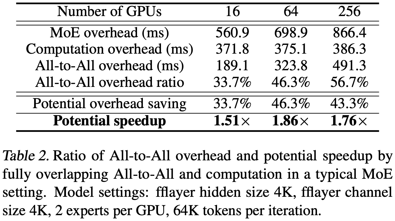
You’d also like to have some other optimizations, like overlapping the token communication with the expert computation. This can net you almost a 2x speedup.
And to make matters worse, you have to worry about utilization for your interconnect. Only large transmits can approach the theoretical throughput.
So to get good efficiency, they add a number of optimizations.
First, they have a better all-to-all operation that reshapes the tensors such that the expert inputs end up in a better layout. It does this by letting you split the input tensor along one dim and concatenate it (once gathered) along another.
Another big optimization is dynamic parallelism. They observe that both sharded data parallelism and tensor parallelism involve each GPU storing one slice of a parameter tensor; this means that, using the same sharding scheme, you can dynamically choose to either move the activations to the weights (tensor parallelism) or move the weights to the activations (data parallelism).
You only have to worry about this switching if there are more GPUs than experts. And it’s pretty simple to choose between them; just use whichever one moves less data.
They also adaptively choose how much to pipeline the communication + computation within a given expert module. I.e., they interleave sending some of the tokens and running those tokens through the experts. This is in contrast to the naive approach of transmitting all the tokens to each expert while the GPUs lie idle and only then starting the expert computations.
To improve communication speed, they implement a hierarchical all-to-all that first coalesces data within each node before sending it to other nodes. To maximize speed, they compile this operator using MSCCL.
Within each GPU, they reduce routing overhead via custom “encode” and “decode” kernels.
Their optimizations make MoE run significantly faster. In isolation, their hierarchical all-to-all can improve communication speed 2x or more for large GPU counts and/or small message sizes.
Their adaptive communication + computation interleaving doesn’t help much at realistic capacity factors (≤2), but it does reliably choose the best available interleaving degree.
Putting everything together, it reduces both runtime and peak memory consumption significantly for MoE layers:
Tutel is a monster of a library and there’s even more in the paper I didn’t get to. But hopefully this gives you a sense for just how much system-level optimization goes into a top-tier mixture-of-experts implementation. MoE is rumored to be a big part of GPT-4, but—given the complexity—it’ll likely be a while before most organizations manage to use it.
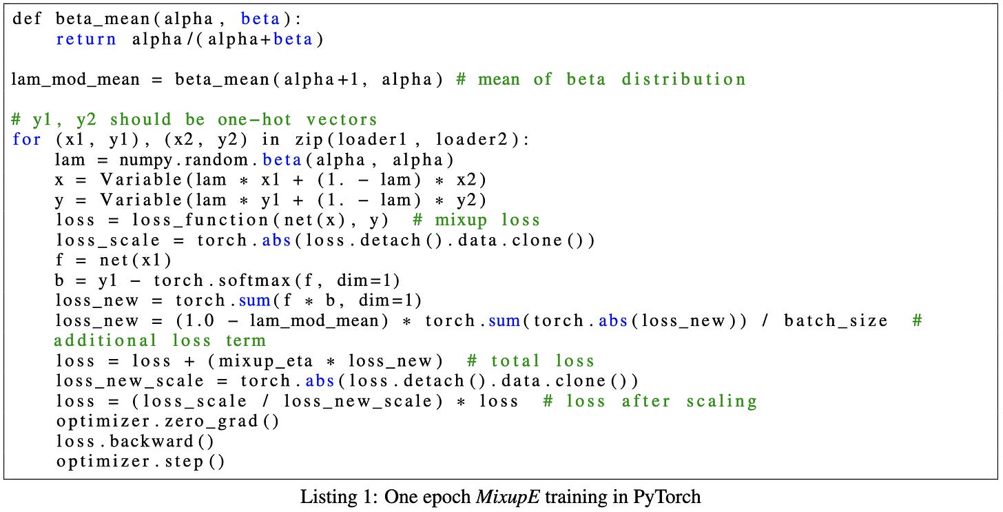
MixupE: Understanding and Improving Mixup from Directional Derivative Perspective
They did a bunch of math to derive a new Mixup variant:
It’s more complex than vanilla Mixup, but seems to regularize harder.
The downside is that it requires an extra forward pass each time. Might be worth trying if you’re working on a problem where more regularization could help.
LAMBADA: Backward Chaining for Automated Reasoning in Natural Language
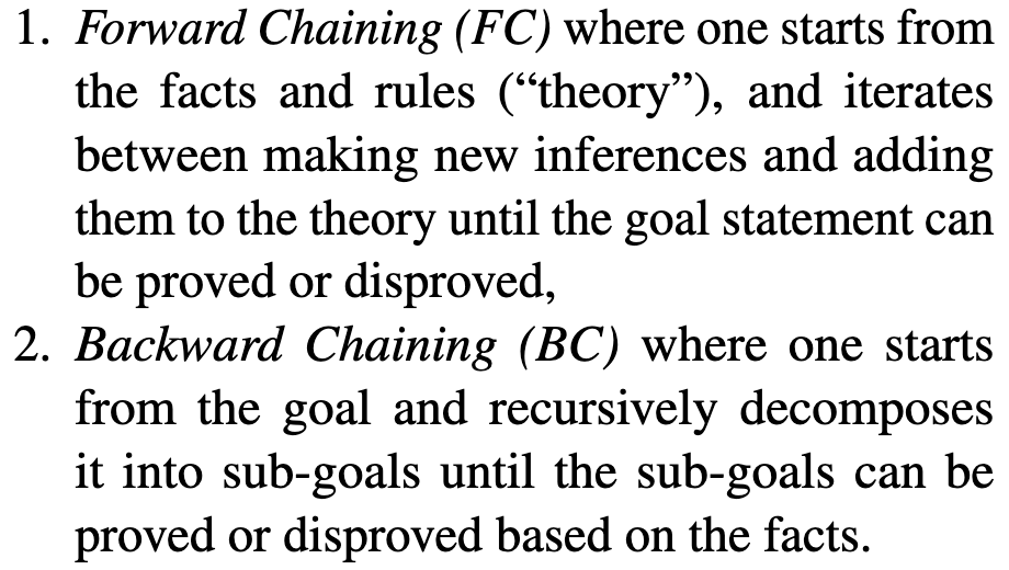
When proving a theorem, you usually use either “forward chaining” or “backward chaining.”
Usually backward chaining works better. So the idea of this paper is to get language models to do backward chaining when reasoning.
They make the model do this by imposing a bunch of structure on its reasoning.
This seems to help it prove theorems better.
Mostly I think it’s interesting that we’re seeing classical AI techniques become relevant again. Feels like we’re headed for a “best of both worlds” situation as our connectionist approaches finally get good at manipulating symbols.
A Theory of I/O-Efficient Sparse Neural Network Inference
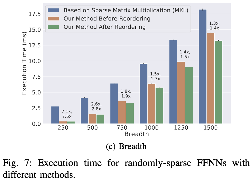
Better unstructured sparse matrix products on CPUs by analyzing the sparsity patterns in different MLP layers ahead of time and maximizing cache reuse. They also prove that their method comes within a factor of 2 of the best possible I/O complexity.
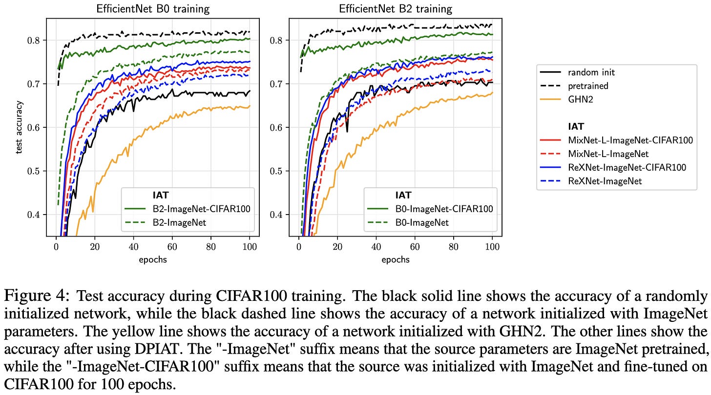
Breaking the Architecture Barrier: A Method for Efficient Knowledge Transfer Across Networks
They transfer parameters from one model to another one with a completely different architecture.
They do this in two steps.
First, they compute a similarity score between each layer in the first model and each layer in the second model. The similarity is based purely on tensor shapes.
Using these pairwise scores, they use dynamic programming to match up the layers. It looks a lot like Longest Common Subsequence or Dynamic Time Warping if you’re familiar with either of those.
This procedure works pretty well, consistently getting a better training time vs accuracy tradeoff than random initialization.
StitchNet: Composing Neural Networks from Pre-Trained Fragments
This paper has me perplexed.
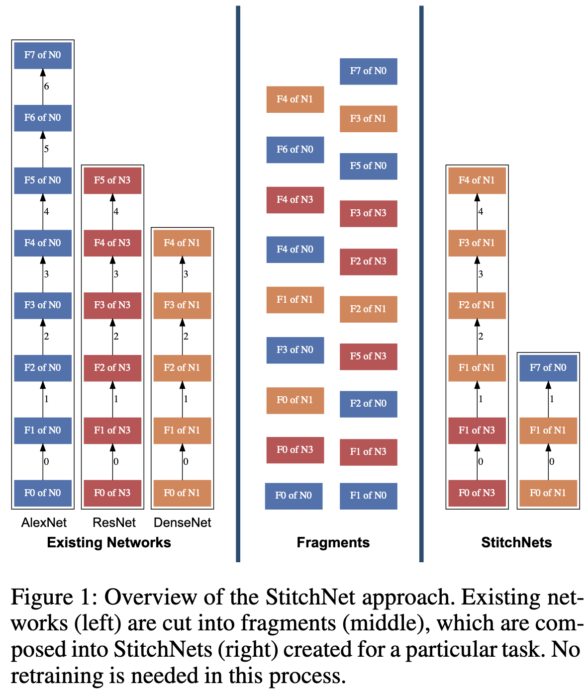
What they’re trying to do is take modules from existing neural networks and combine them together to get a new neural network for a more specialized task. E.g., throughout the paper, they transfer ImageNet networks to the Cats vs Dogs dataset.
Their procedure for doing this is:
Start with the first layer from one of their source networks as the initial model.
Iteratively compute a similarity score between the output distribution of the network-so-far and the input distribution of every module in every source network (evaluated within the source network). The distribution is assessed using the same inputs in the same order across all networks. The similarity they use is Centered Kernel Alignment.
Choose one module to append, taking into account the similarity score, runtime, parameter count, and whatever else you want.
Use ordinary least squares to linearly transform the current last module in your network such that its outputs have minimum L2 distance to the appended module’s inputs.
When you append the final layer of one of the source networks, you’re done. If the original and target output spaces are different, you can manually map existing classes to your classes of interest (e.g., they throw away all the imagenet classes that aren’t cats or dogs).
Here’s the pseudocode:
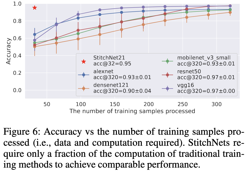
The impressive result here is this. For a fixed number of samples, they find that they’re better off constructing a StitchNet than finetuning any of the original models. In the former case, the samples just serve to estimate and align the input and output distributions for all the layers—no finetuning involved.
This result is…really weird, for several reasons:
There’s nothing in the StitchNet procedure that encourages accuracy—only similarity of intermediate representations.
If you take the output with the highest similarity score at each iteration, I’m pretty sure the resulting StitchNet will always be the original network whose input module you started with.
In my experience, even the slightest change to a pretrained image classifier (e.g., pruning 10% of the weights) will hurt the accuracy a lot if you don’t finetune to compensate. So finding that a mashup of multiple networks does not merely as well as the original networks, but better than finetuned versions of those networks is…really surprising.
So I’m not sure how well these results will generalize to other tasks, but this paper definitely violates my mental model of neural net training (a good thing!) and suggests that more compositionality might be possible than previously thought.
Machine Learning Containers are Bloated and Vulnerable
Even Docker containers provided by Google, Meta, and NVIDIA are larger than they need to be. Below, the “bloat degree” is 0 if the container can’t shrink at all without breaking and 1.0 if everything in it can be removed.
This wasted space translates to slower container pulls and job launches.
Thanks mostly to the bloat, these containers also contain a variety of known security vulnerabilities.
Semi-relatedly, they have this cool visualization of the lines of code in PyTorch and TensorFlow. In case you didn’t realize it, these frameworks are multi-million-line behemoths.
Discovering Language Model Behaviors with Model-Written Evaluations
A big old LLM paper from Anthropic.
Basically, instead of having humans collect / create evaluation datasets, they have LLMs generate them. They do this by splitting dataset generation into various steps, often including filtering.
The resulting datasets are about on par with human-generated datasets, at least as evaluated by crowdworkers (eval not shown below).
Using the 154 datasets they generate, they assess all sorts of aspects of their models, including how techniques like RLHF affect their outputs.
They even evaluate properties related to worst-case AI risk.
Relatedly, this snippet makes me suspect that discussion of AI risks is a self-fulfilling prophecy. Like, maybe this thing is reasoning about causation and independently concluding that it can’t do its job if it’s shut down—or maybe it’s just parroting the countless EA forum and Less Wrong posts talking about how AIs will do this.
Super thorough work that suggests we might get a virtuous cycle of language models being good enough to generate more training data for themselves (or at least more evaluation data).
Unnatural Instructions: Tuning Language Models with (Almost) No Human Labor
They have a pretrained language model generate a big dataset for instruction tuning using just a handful of initial instruction-input-output examples. In case you missed it, instruction tuning means finetuning your language model on example prompts + high quality outputs (as opposed to just random documents). And it can yield huge accuracy gains.
More precisely, they start with a prompt like this and have the model generate a new instruction, input, and set of constraints. They keep all the responses that pass some sanity checks—e.g., having all the requisite fields and not verbatim copying the prompt.
One limitation of these structured instruction-input-constraints texts is that they’re kind of unnatural and formulaic. To get more diverse and natural-sounding examples, they have the model paraphrase them.
You may have noticed that we haven’t generated the “ground truth” outputs for our examples yet. To get these, they just feed the instructions, inputs, and constraints into a pretrained model and use its output as the ground truth.
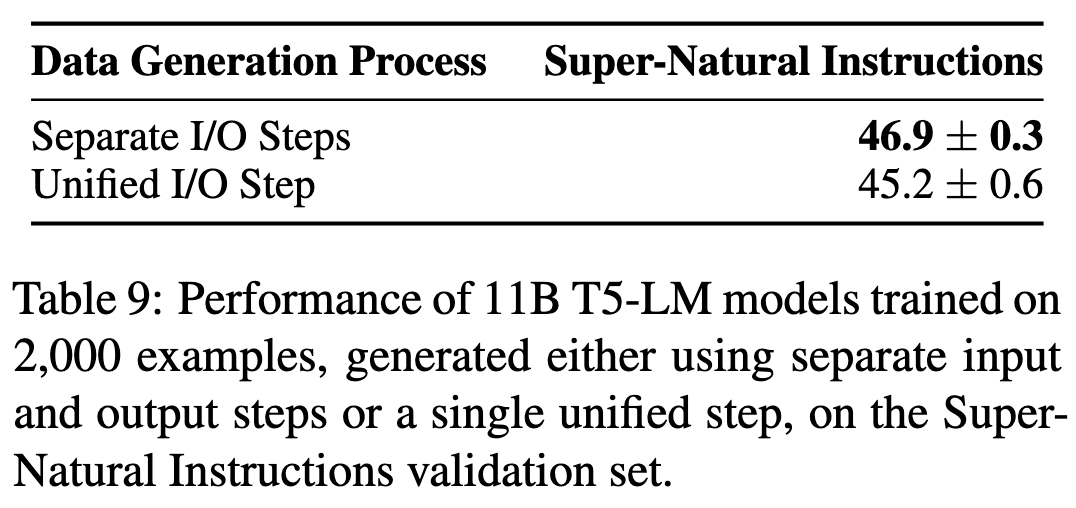
They decouple the input generation and output generation for each example since that works better. They suggest that this is because they need stochastic decoding to get diverse inputs, but greedy decoding works better for choosing the most likely output.
Putting these steps together, you get examples that look like this (where “{INPUT}” gets filled in with the “Input: ” field from another example).
Using this procedure, they construct the Unnatural Instructions dataset. As you can see in the bottom row, finetuning T5 on this dataset does almost as well as finetuning on larger human-created datasets.
On a per-sample basis, you’re better off using handcrafted instruction tuning data (the Super-Natural dataset). But on a per-dollar basis, their data generation procedure is way cheaper than paying crowdworkers.
Importantly, their results also seem to get better when the models generating the example inputs and outputs get more sophisticated. This suggests a virtuous cycle of smarter language models yielding better training data yielding smarter language models.
Between this and the previous paper, it feels like language models creating their own data is about to be a mainstream thing. Since high-quality data being expensive has been so fundamental to ML and statistics for so long, I’m not even sure what all the implications of this will be…


