2022-12-4 arXiv roundup: New best MoE implementation, 3x faster transformer inference
This newsletter made possible by MosaicML.
MegaBlocks: Efficient Sparse Training with Mixture-of-Experts
They cast MoE modules as block sparse operations and use this framing to speed up MoE by a lot in the num_experts > num_devices regime.
More precisely, they point out that you can look at an MoE layer as an activation-sparse matmul. Each expert corresponds to a group of columns that are nonzero together, and top-k routing assumes that k groups of columns are nonzero for a given token.
Based on this framing, they write block-sparse CUDA kernels that perform the operations in an MoE with way less overhead than typical implementations.
In particular, they get to throw away the capacity factor hparam. This factor is the amount of padding you do to deal with the imbalance in how many tokens get assigned to each expert. Normally, you need quite a bit of padding to get full accuracy.
To replace the capacity factor, they just determine the block-sparse structure dynamically for each back of tokens, doing exactly the amount of work required for each expert.
This approach allows them to train models much faster than the current fastest MoE implementation (Tutel) as well as the baseline non-MoE model.
Also, they did an awfully good job writing the kernels. They get throughputs with their block-sparse matmuls on par with cuBLAS BMMs of equivalent shapes.
This is probably the best MoE implementation there is right now, especially since it lets you avoid setting the capacity factor.
I also wonder what else one could do with input-dependent block-sparse kernels that run at the speed of similar dense ops. Feels like it opens up possibilities for more sparsity research that actually improves wall time.
Fast Inference from Transformers via Speculative Decoding
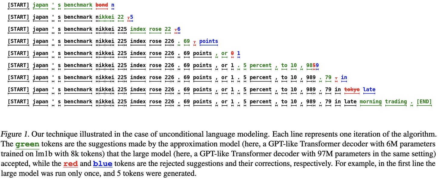
They use speculative execution to sample multiple tokens from each forward pass through your text generation model. And more impressively, they do this without changing the sampling distribution.
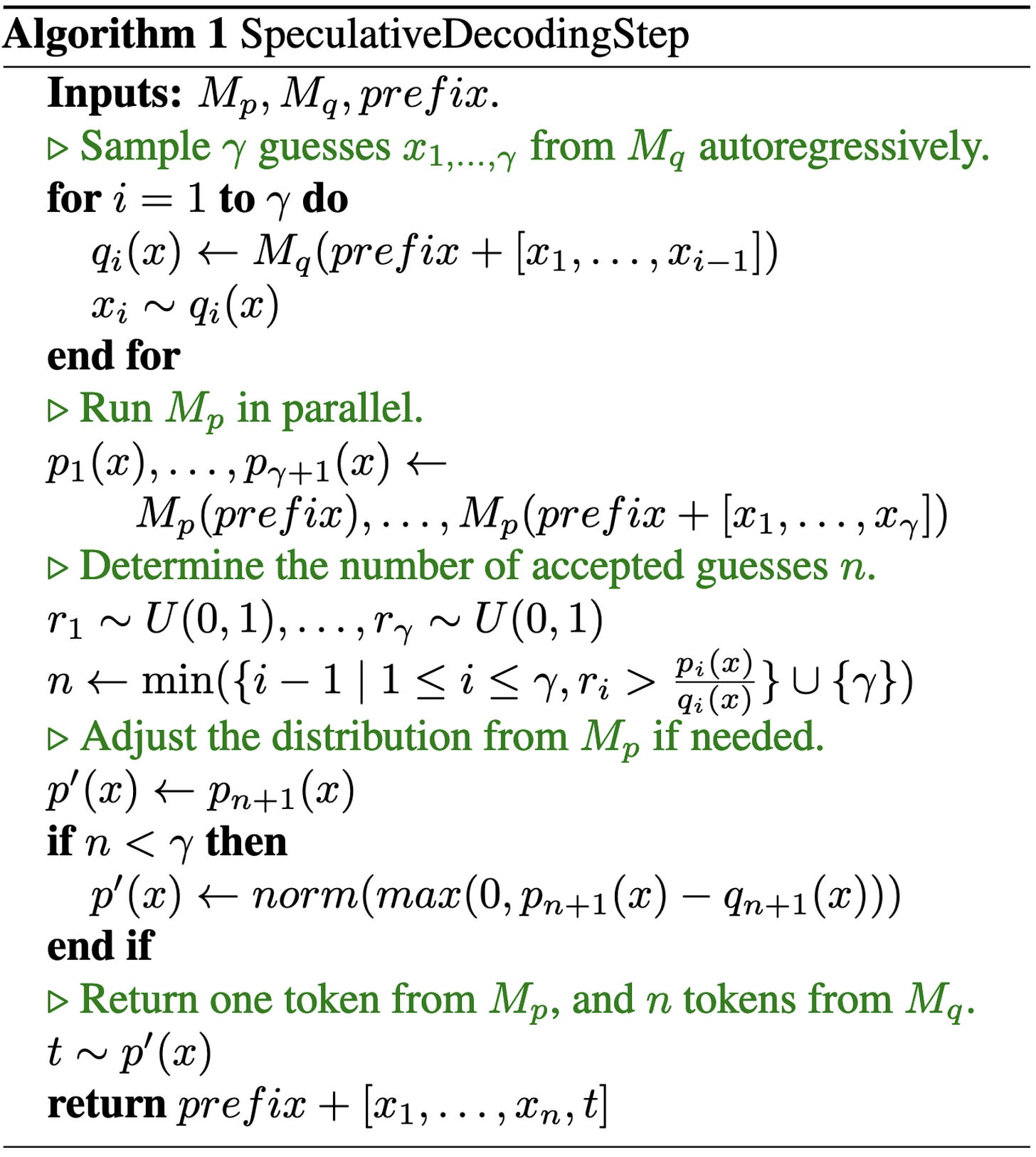
The idea is super clever and exploits a property of rejection sampling. Let p(x) be the distribution over the next token from the true model and q(x) be the distribution from a smaller, cheaper model. You can sample from p(x) exactly by:
Generating a sample from q(x)
Accepting it whenever q(x) < p(x)
Accepting it with probability p(x) / q(x) whenever q(x) > p(x)
The key here is that we can do (1) cheaply and defer (2) and (3) until later. This lets us iteratively sample a token from q(), condition on this token to get q() for the next token, sample another token, and so on, guessing several tokens into the future.
Once we’ve guessed a bunch of future tokens, we can feed this whole conjectured sequence into our real model at once. Because generating one token at a time tends to get poor utilization, we can feed in the whole predicted sequence for nearly the same cost as doing one token at a time. Moreover, in the case that the whole speculative sequence is accepted, this costs us no extra FLOPs.
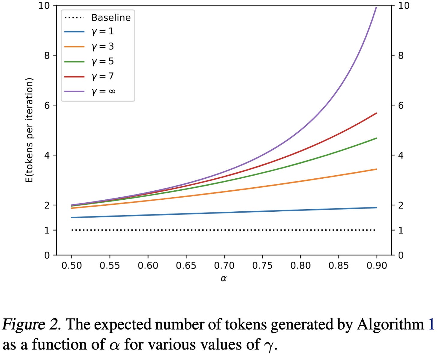
Letting α denote the expected acceptance rate and γ the number of tokens ahead we try to generate, the expected number of tokens generated per forward pass is:
This induces a tradeoff between making q() and p() similar and making the q() model cheap to run. For a given average acceptance probability and marginal cost per token in the forward pass, it also induces an optimization problem with respect to γ.
Their method lets them run T5 inference 1.5-3.5x faster. This is a huge gain, especially considering that there’s zero loss of accuracy.
I’m a fan of this method. Partially because of the great results, but also because it’s rare to find a paper that offers a new algorithmic tool to work with; I feel like “stochastic speculative execution” via rejection sampling might be useful in many more contexts.
Efficient Training of Large Language Models Using Pipelining and Fisher Information Matrices
Second-order optimizers converge in fewer steps, but require a bunch of extra computation to update their preconditioning matrices. Pipeline parallelism induces “bubbles” in which accelerators sit idle. Why not use the bubbles to compute the preconditioning matrices? This lets you get the convergence rate of second-order optimizers without the overhead.
Below is their scheme in a bit more detail, along with the single-GPU and data-parallel baselines. Note that, with data parallelism, the second-order optimizer requires allreducing not only the weight gradients, but also the activations and output gradients. After these allreduces, though, you can shard the matrix inversion work across devices (“inversion parallelism”).
To get the ideal schedule of forward, backward, communication, matrix inversion, and param updating, they profile many options offline and then reuse the best schedule throughout training. The result is pretty high utilization, at least at small scale—~89% with 1 GPU per stage and ~86% with two GPUs per stage.
They also try adding their method onto Chimera, one of the more promising pipeline parallelism schemes. With this more exotic scheme on 8 GPUs, they get up to 97.6% utilization. I’m not sure how they’re measuring utilization though because the matmuls themselves won’t attain this fraction of peak throughput—probably just looking at the fraction of the time some kernel is running.
Overall, they can accelerate training ~2x relative to using the LAMB optimizer with unmodified Chimera pipeline parallelism.
This is one of those papers that makes me feel like, “oh yeah, of course you should do it that way. Why didn’t I think of that?” I mean this in a good way—it indicates there’s a real insight behind it.
Spatial Mixture-of-Experts
Instead of having data-dependent routing, they route based only on the spatial location. This makes sense for tasks like weather prediction where spatial positions have consistent meanings. They also route each spatial position separately (one pixel per token, not one patch). And they do weighted concatenation of outputs from different experts rather than weighted sums.
Two other unconventional aspects are their routing loss and “error dampening.” The former treats routing as a binary classification problem, with labels supplied by whether the gradient wrt the layer’s output at a given pixel is in too high a percentile (with “too high” defined by an hparam). The error dampening consists of scaling down the gradient whenever a routing assignment is “incorrect” according to the above label. The idea is to not update experts based on inputs that shouldn’t have been routed to them in the first place.
Their routing function and loss dampening seem to help, and result in a model that does better than alternatives on some spatial datasets.
Interesting method of baking in spatial inductive biases. We usually see people trying to achieve spatial invariance, so it was a good exercise reasoning about the opposite problem.
Wild-Time: A Benchmark of in-the-Wild Distribution Shift over Time
They introduce a benchmark for handling temporal shifts, a special case of distribution shifts caused by the passage of time (and often featuring timestamps).
Galvatron: Efficient Transformer Training over Multiple GPUs Using Automatic Parallelism
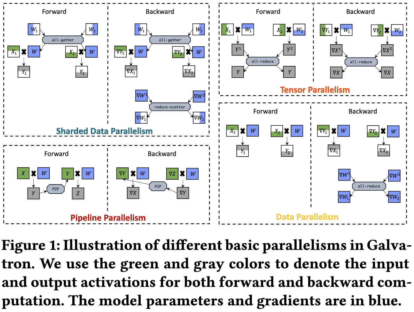
They observe that you can compose all sorts of different parallelism at different scales. E.g., you can do pipeline parallelism across nodes and hybrid data + tensor parallelism within a node. This results in a huge search space for parallelism strategies.
To explore this search space, they decompose it into a tree of decisions about which parallelism to add in next and what world size it should use. They also use dynamic programming to build up a global solution based on the solutions for each submodule. The throughput estimation for each proposed solution uses a mix of profiling and simulation.
They introduce two simplifications to reduce the search space. First, they always make pipeline parallelism the “outermost” strategy. Second, they only allow each parallelism type to show up once (e.g., no tensor parallelism on top of data parallelism on top of tensor parallelism).
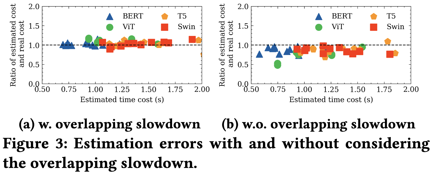
There are a couple subtleties in doing the throughput estimation right. One is that communication and computation can often be overlapped. Another is that you might need to change the tensor layouts across different ops when they use different parallelism strategies.
Putting it all together, their method obtains higher throughputs than Megatron, Deepspeed, FSDP, and vanilla DDP across a variety of transformers.
The main downside is that there’s extra search time at the start. Although this should be minimal relative to the cost of training.
In case you’re curious, here are some example parallelism strategies that it selects. What I find most important here is that it almost never selects just one type of parallelism—you want an optimal mix of moving activations and data, not just one or the other.
I’ve been thinking about the marginal value of hybrid parallelism on a per-tensor level and it’s great to see someone prove out the benefits. I was also surprised to see how much variation there was among parallelism strategies/libraries—it was often a >2x speed difference, despite them all using the same model on the same hardware.
PAC-Bayes Compression Bounds So Tight That They Can Explain Generalization
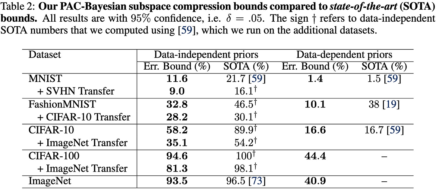
They get generalization bounds on various models that are actually not that far from empirical validation accuracies.
They also get better bounds when starting with a pretrained model or baking in invariances, and worse bounds when the data is noisier. these are all consistent with empirical behavior.
Their key idea is to restrict the size of the hypothesis class H through compression. This lets you get a provably small difference between the training risk and test risk as your sample count n increases.
To get tighter bounds, they lean on existing results that let you use a prior over the hypothesis class and sample a single hypothesis (at the cost of instead bounding expected risk).
The first part of restricting the hypothesis space is applying only low-rank updates to the weights. In the finetuning case, they do this by only training the batchnorm and last layer parameters. For pretraining, they also allow a Kronecker factorization of the weight changes.
To reduce the hypothesis class further, they quantize the model and then arithmetic code the quantized weights.
They argue that their results help explain generalization. E.g., their findings suggest that overparametrization doesn’t hurt you as long as you can get away with lower-dimensional updates. Similarly, when there’s less structure in the dataset, you need higher-dimensional updates (which yield worse generalization).
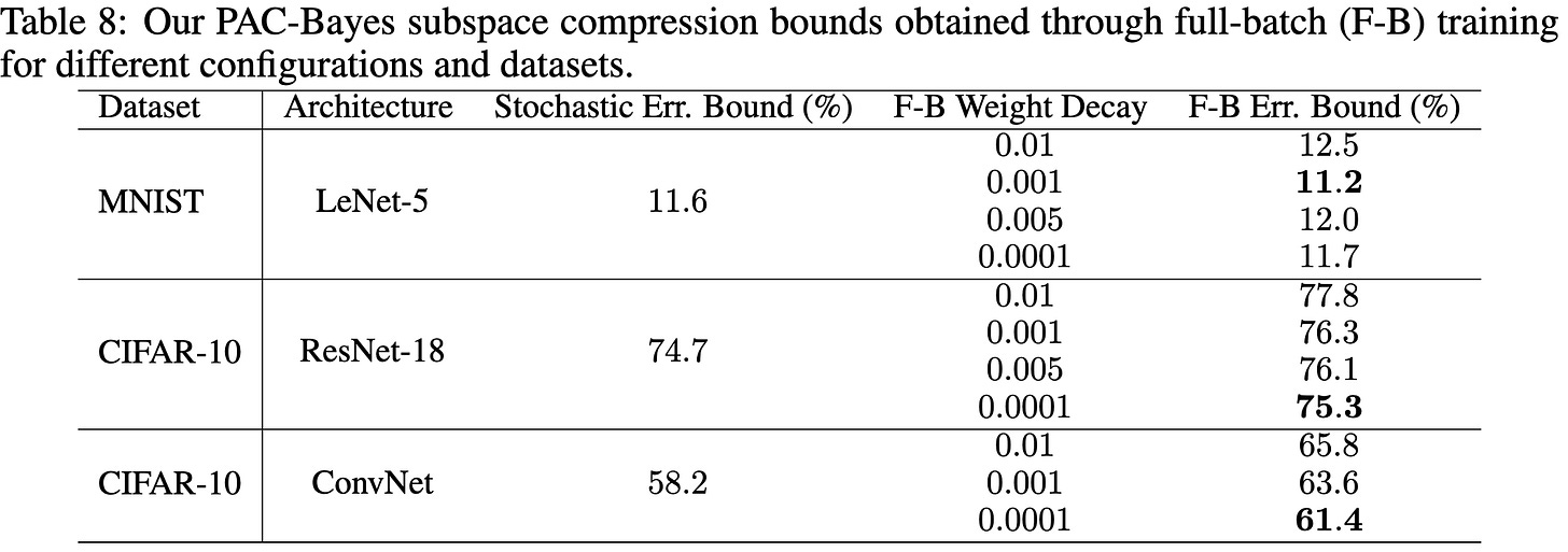
By performing full-batch training and still getting decent generalization guarantees, they also demonstrate that the stochasticity of SGD isn’t necessarily the main explanation for neural nets generalizing.
I don’t follow the deep learning theory literature closely, but this feels like an important result. And it makes me wonder how much farther we could push the numbers with better model compression. E.g., what if we used vector quantization instead of scalar quantization, bzip2 instead of arithmetic coding, or even expensive neural compressors instead of classic compression algorithms?
Traditional Classification Neural Networks are Good Generators: They are Competitive with DDPMs and GANs
Image classifiers output class predictions, not images. But they do learn a fair amount about their input distributions. Can we use this knowledge to generate images from a trained classifier?
The answer is yes. The basic idea is to start with a random image and iteratively update it based on the activations and gradients it induces in the model. But this is hard. Most existing work that does this ends up getting crazy psychedelic images, not realistic ones.
To make this work, they essentially use the original classifier as the backbone for a masked autoencoder. They also add some changes like progressively increasing the image resolution and using a loss that encourages diverse samples.
Works fairly well, although definitely likes to tile the same texture all over the image.
Interesting that this works. Probably won’t replace regular image generation models anytime soon, but suggests it might be possible to interrogate what a vision model knows using new output spaces—sort of like adding a linear probe, but easier to visualize.
Finding Differences Between Transformers and ConvNets Using Counterfactual Simulation Testing
They release the Naturalistic Variation Object Dataset (NVD), which consists of simulated views of tons of objects from different perspectives with different lighting conditions and occlusions. The images are generated in Unity via ThreeDWorld.
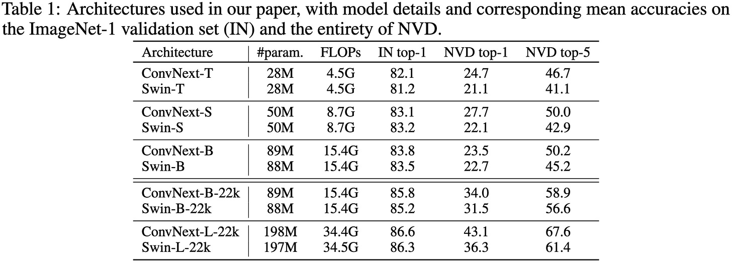
They use this dataset to study the properties of parameter and FLOP-matched ConvNexts and Swin transformers.
Swin transformers are better at dealing with occlusions, especially large ones.
But ConvNext is often better at dealing with variations in object scale,
camera viewpoint,
and object rotation.
This is one of the most apples-to-apples comparison of CNNs and transformers I’ve seen. It’s not obvious to me why these differences in robustness hold—e.g., why would shift invariance buy you better pose invariance? But often that sort of intuition-violating result is what leads to better understanding down the road.
Finetune like you pretrain: Improved finetuning of zero-shot vision models
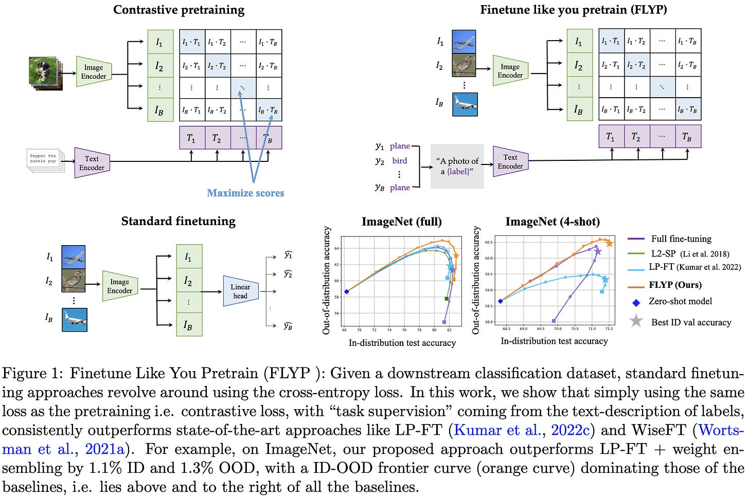
They propose to finetune image classifiers using a contrastive loss similar to that of CLIP pretraining.
Basically, given a pretrained language model, you try to make the embeddings of text like “A photo of (label)” be 1) the same as the embedding for that image, but 2) different from the embeddings for other images in the batch. Note that they also finetune the language model as they go and this seems to help.
This approach outperforms a variety of other finetuning approaches both in-distribution and out-of-distribution, including good old cross-entropy loss.
The gains are especially large when there are only a few labeled samples per class.
They provide evidence that the gains stem partly from exactly matching the pretraining objective. In particular, making the loss not penalize similarity between embeddings for the same class doesn’t help like you’d expect. This is counter-intuitive since images from the same class are supposed to have identical embeddings, so why would we penalize that?
What I’m most curious about here is whether this beats cross-entropy with label smoothing, PolyLoss, or other cross-entropy variants (which avoid the overhead of also finetuning a text encoder). If so, I could see this becoming a best practice.
SPARTAN: Sparse Hierarchical Memory for Parameter-Efficient Transformers
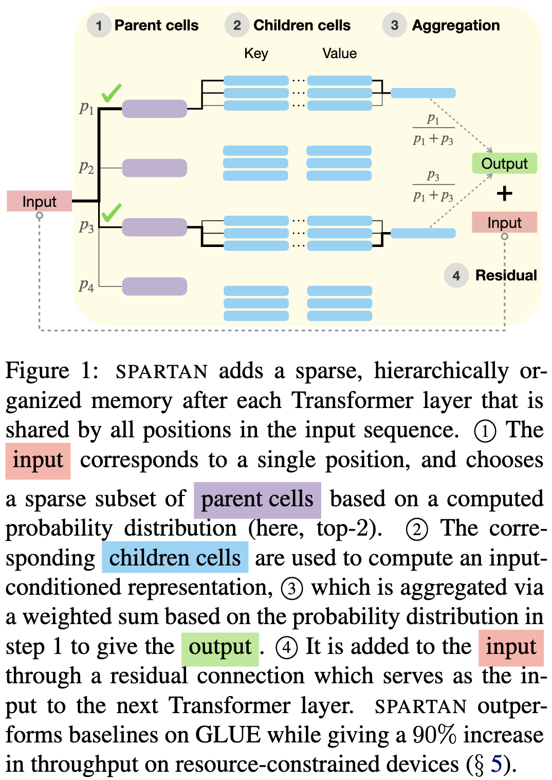
They add a trainable key-value store after each transformer block. The keys and values are grouped together and each group is associated with a “parent” vector. The output is a weighted sum of the values in top k groups, with each value’s weight proportional to both:
the inner product between the input and the parent,
the (softmaxed) inner product between the input and the key
It’s basically a mashup of a vector search index and a regular differentiable kv store. You can also look at this as a hierarchical MoE model where each expert returns a constant instead of performing a matmul.
Seems to have a much better throughput vs accuracy tradeoff than other methods on mobile devices, though not better than a regular RoBERTa. It is much smaller than RoBERTa though (presumably because they’re starting with a smaller baseline model?).
The Effect of Data Dimensionality on Neural Network Prunability
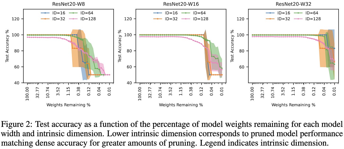
Does higher-dimensional input data make it harder to prune your image classifier? Depends on your definition of “higher dimensional.”
If you just change the resolution of your images, the answer is mostly no. Both reducing and increasing the resolution of CIFAR-10 relative to the original 32x32 size decreases absolute accuracy, but doesn’t really affect the shape of the accuracy vs sparsity curve.
If you instead consider intrinsic dimensionality, the story changes. Having higher intrinsic dimensionality in your images makes pruning less effective. Here, intrinsic dimensionality is the size of the latent space for a GAN used to generate the images.
Lastly, what about “task dimensionality,” defined as the number of input features that convey information about the output label? Using a similar GAN setup, they find that this has no effect on prunability.
Small-scale experiments, but really clean questions, explanations, and results. I wish more papers were this easy to understand.


