2022-8-14 arXiv roundup: Branch-Train-Merge, Model patching, lots of LLM papers
This newsletter made possible by MosaicML.
Branch-Train-Merge: Embarrassingly Parallel Training of Expert Language Models
They got training to be both way faster and way more modular, to the extent that it might change standard practice for training models.
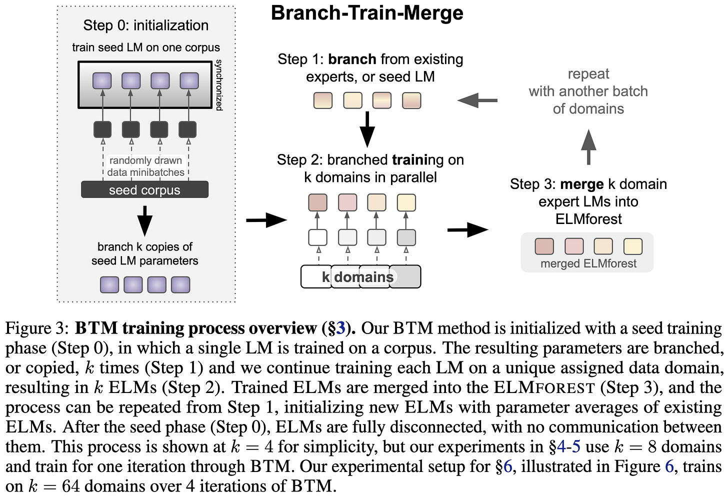
The idea is, instead of training one model for all your text data, you train a different model for every “domain” in your text and ensemble them. E.g., one model for legal documents, one for arXiv papers, etc. Because these models can be trained independently, training becomes embarrassingly parallel.
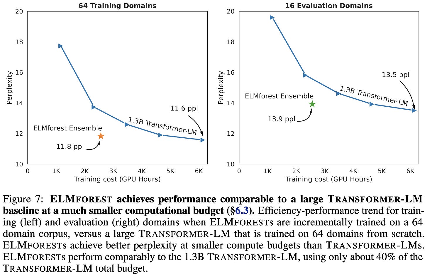
What’s surprising is that this works really well, in this sense of getting you both much lower perplexity and much faster training.
This holds from 8 “domains” (above) all the way up to 64 domains (below).
Now, it doesn’t seem to be the case that this “just works” with a naive approach. They propose a specific procedure for initializing the different models, handling optimizer states, and weighting models in the ensemble.
One big ingredient is spending some fraction of the training budget on creating a “seed” model that uses data from many domains. Fortunately, it doesn’t matter too much what fraction of the budget you use for the seed model as long as it’s not all of it.
Given this seed model, they “branch” off different copies of it, and train each copy on a different domain. Once the copies are trained, they merge them into one model. This can mean either ensembling them all with intelligent weighting, or just plain averaging all the models’ parameters. Ensembling yields lower perplexity but has inference overhead proportional to the number of models.
I’m more bullish on the parameter averaging due to the reduced inference overhead—seems like a stronger version of Model Soups.
Overall, super interesting work that offers a path to more parallel, modular training, as well as a lot of food for thought regarding how we do mixture of experts.
Memory Performance of AMD EPYC Rome and Intel Cascade Lake SP Server Processors
Ever wonder what’s actually different between Intel and AMD CPUs? This paper digs deep into the architectures of AMD EPYC Rome and Intel Cascade Lake processors.
First, the overall interconnect of the processors is different. The AMD processor is somewhat tree-structured, with 8 compute chips (CCDs) plugged into a 9th I/O chip.
And within each compute chip, there are two groups of up to 4 cores. Each of these groups has a 16MB L3 cache. Pairs of these chips are associated with a NUMA (Non-Uniform Memory Access) node, meaning that 1/4 of the DRAM is faster to access for each core than the rest of DRAM.
Meanwhile the Intel processor is a single chip with a mesh interconnect, where each element of the grid can talk to its neighbors in the same row or column.
The L3 cache is shared across the whole processor and sharded across all cores, rather than unique to a group of 4 cores.
Within each core, the AMD chips have half the L2 cache size, L2 cache bandwidth, and vector instruction width compared to Intel chips. Although they find in microbenchmarks that the AMD chips come closer to achieving their theoretical peaks.
Besides just describing the architectures, they run a ton of microbenchmarks. As one might expect given the tree vs mesh interconnect, Intel’s worst case read latencies are lower than AMD’s.
There’s a similar gap in tail latencies for communication across sockets (i.e., across CPUs in the same server).
However, they do find “a 41 % lower RAM bandwidth for an entire socket
for the [Intel] processors compared to Rome” thanks to the former having only six memory channels rather than eight. This suggests that AMD chips might be better suited to embarrassingly parallel, memory-bound workloads.
For deep learning, these findings are pretty consistent with my experience. It wasn’t quite apples-to-apples, but we found at one point that we had to double the number of dataloader workers for ImageNet training when switching from Intel to AMD chips. Though, to be fair, this was possible to do because the AMD chip had twice as many cores. I’ve also seen evidence that recent Intel chips do better on number crunching benchmarks outside of data loading.
Regularizing Deep Neural Networks with Stochastic Estimators of Hessian Trace
They add the estimated trace of the Hessian as a penalty term to the loss.
They get this estimate using Hutchinson’s method, which roughly consists of averaging many Hessian-vector products with 0-mean random vectors:
This ends up looking as follows:
Except they fuse in dropout regularization by masking the random vectors to add extra regularization.
This technique seems to increase accuracy a fair amount on CIFAR-100:
I think this requires a second backwards pass, meaning it might not be worth it from a training time perspective. But there are also so many methods now that require a second backwards pass (e.g., SAM and most of its variants, AdaHessian) that I wonder if just always doing two backwards passes will become standard. Though it remains to be seen how well such methods compose with one another.
Quality Not Quantity: On the Interaction between Dataset Design and Robustness of CLIP
How well will image-text models trained on a given dataset generalize to a different dataset?
The answer is: it’s complicated. Different pretraining datasets work better for different downstream datasets.
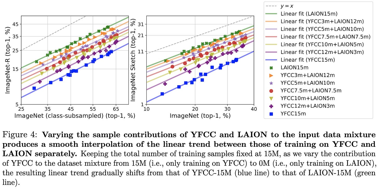
One interesting but inconvenient result is that mixing more upstream datasets doesn’t necessarily work better. It’s more that other datasets dilute the robustness imparted by the best dataset.
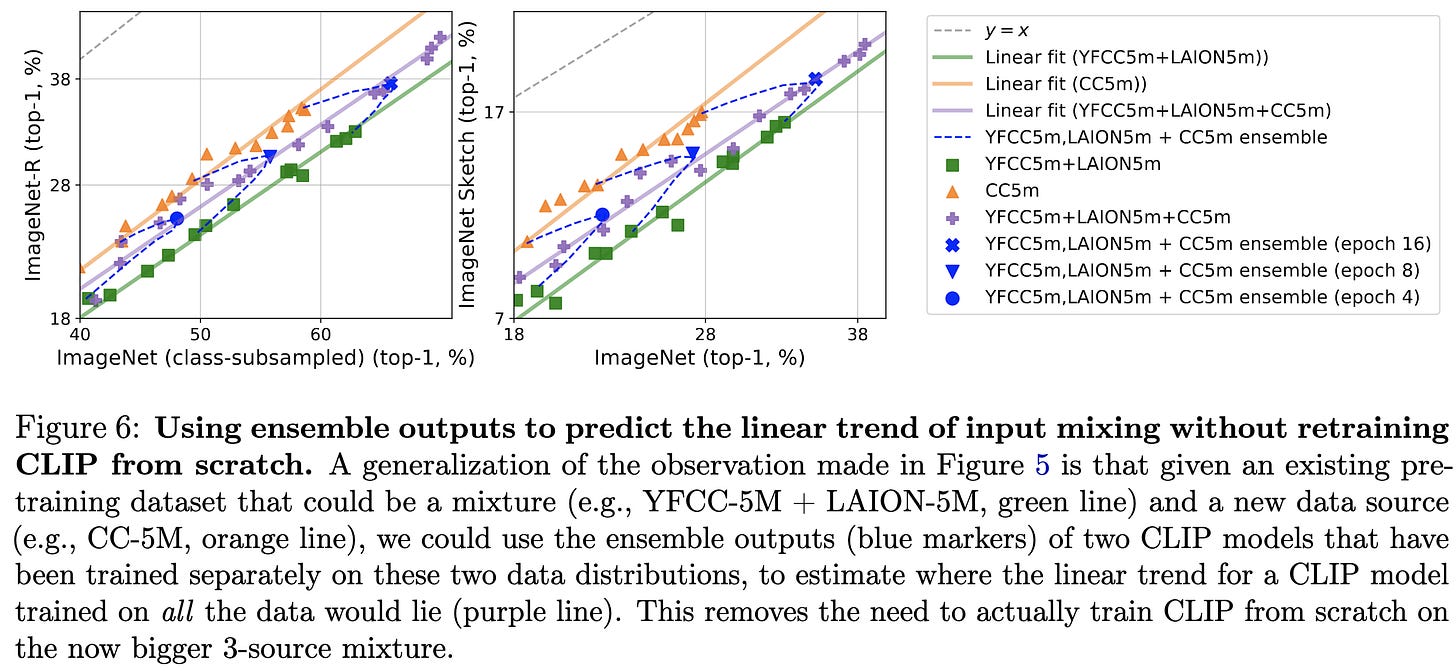
But the good news is that you can use a model pretrained on a given dataset as a proxy for that dataset. In particular, rather that train on convex combinations of datasets, you can take convex combinations of the predictions from their associated models to estimate downstream performance.
You can take this even further and estimate trend lines for how well a model would perform given more data using just the predictions of the pretrained models for relevant dataset subsets.
Among other things, these findings highlight the importance of using multiple downstream tasks when assessing the quality of a pretraining dataset.
My mental model for pretraining datasets after reading this is that yes, more data is more—but the relevance of the pretraining dataset is much more important than its diversity; you get way more benefit from having one highly relevant corpus than many low-relevance ones. So much so that, given fixed pretraining compute, you might (?) be better off pretraining separate models for different downstream tasks rather than one big one. This is a pretty different paradigm than what most people seem to be assuming.
Also—wow, these trends are so linear. We’ve seen this in several papers now, so linearity in transfer accuracy seems to be a real thing.
Language Tokens: A Frustratingly Simple Approach Improves Zero-Shot Performance of Multilingual Translation
To make translation models work better, tell them both the source and the target language in the encoder input and tell them target language in the decoder input.
This approach has about the same or greater effectiveness when translating English, but works much better when translating directly between non-English languages.
Another example of the importance of prompt design. Makes me wonder three things:
Should we just pack the prompts with all the features and metadata we possibly can?
Is there a compute-optimal prompt length vs model-size tradeoff?
Is handling longer, richer prompts the killer app for subquadratic attention?
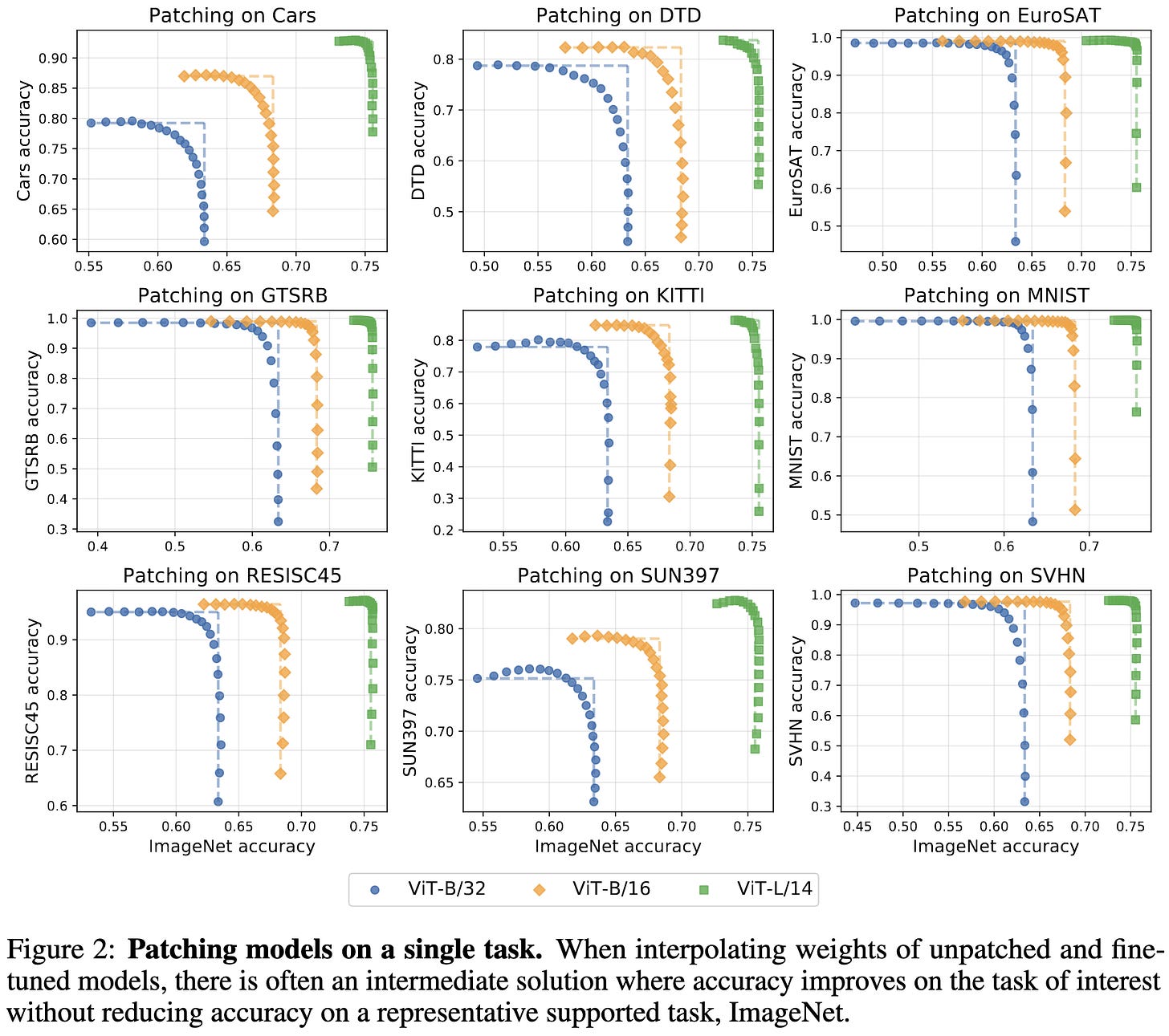
Patching open-vocabulary models by interpolating weights
Taking a convex combination of pretrained weights and finetuned weights for a given downstream task you give you a strong tradeoff curve of original task accuracy vs downstream task accuracy.
You can get a large lift in downstream accuracy for almost no reduction in original task accuracy.
Larger models can be patched more easily, probably because of the curse/blessing of dimensionality. I.e., random weight perturbations will tend to become orthogonal to the gradient direction on the original data as the dimensionality of the weights increases.
It also appears that simple linear interpolation is the best approach. You can try fancier schemes, but good old interpolation recovers the Pareto frontier.
If you want to patch a model to support multiple new downstream tasks, you should jointly train on all of them and patch once if possible. The fact that sequential patching works better than parallel matching suggests to me that the directions of the weight perturbations aren’t quite orthogonal, and/or that the local curvature matters.
Patching can sometimes yield positive transfer to tasks you didn’t even patch on. E.g., patching on a synthetic task can make your model more robust to typographic attacks.
Overall a really thorough and interesting paper that serves as testament to the power of linear mode connectivity.
Simplified State Space Layers for Sequence Modeling
A successor to S4 that replaces separate state-space models for each input dimension with one shared state-space model of lower rank.
This formulation lets them simplify the layer a fair amount. Basically, their formulation lets them diagonalize the transition matrix, which means they can just do elementwise multiplies at each time step. Combined with a fast parallel prefix scan, they can quickly process the whole input sequence.
Seems to yield about the same accuracy as S4. Unclear what the runtime story is, but both approaches have fairly similar complexity.
If you really want to understand what’s going on here, I would definitely recommend reading the JAX implementation in Appendix A. But one takeaway is that there exist S4-like replacements for attention other than the specific polynomial approach used in S4.
Controlled Sparsity via Constrained Optimization or: How I Learned to Stop Tuning Penalties and Love Constraints
It’s really hard to tune penalty terms to give you a target level of sparsity, so you should just hard constrain the amount of sparsity instead.
I strong agree here; this is consistent with basically all the sparsity stuff I’ve ever done. There are tons of ways of finding your nonzeros given a hard constraint (see, e.g., lots of compressed sensing literature), and this paper proposes one based on elementwise learned gates that seems to work pretty well.
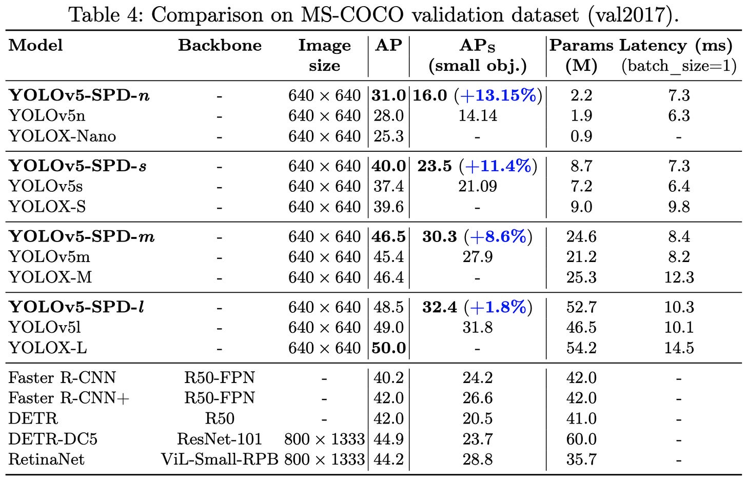
No More Strided Convolutions or Pooling: A New CNN Building Block for Low-Resolution Images and Small Objects
Instead of using a pooling layer or having a stride for your conv, just use a space-to-depth op.
This substitution seems to usually be an improvement, even conditioning on inference latency. This is especially true for small models and when detecting small objects.
My current mental model of space-to-depth is that it
throws away translation invariance (bad),
is bandwidth bound if you do it along both rows and cols (bad), but
preserves all the information (good).
I’d love to see more experiments comparing to BlurPool and/or some characterization of how the runtime changes when not also multiplying the next conv’s input channel count by 4x.
Why Do Networks Need Negative Weights?
Answer: if they don’t have negative weights, they might not be universal function approximators.
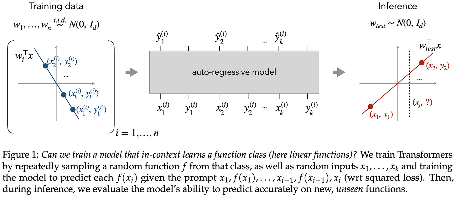
What Can Transformers Learn In-Context? A Case Study of Simple Function Classes
In-context learning is when you include some examples as text in the prompt. How fancy can we get with these examples?
It turns out you can get a GPT-2-like model to learn a linear function almost as well as an actual least squares solver. And this is without teaching it anything about least squares directly—just giving it (x, y) samples.
The model also works about as well as least squares on OOD data.
It can also learn more sophisticated function classes like 2-layer MLPs, sparse linear models, and decision trees. And it does so better than various strong baselines.
Unsurprisingly, in-context learning works better with larger models and easier function families. It also works way better if you design a curriculum of increasingly difficult function families during the training, rather than training just on the full difficulty.
Really surprising that this works so well, and mildly surprising that curriculum learning was so impactful (since it usually isn’t).
Efficient Training of Language Models to Fill in the Middle
What if you want your generative language model to be able to output text in the middle of a sequence instead of just at the end? E.g., in OpenAI’s case, they want to suggest code where your cursor is instead of just at the end of the function.
They propose Fill-In-the-Middle (FIM) training, which consists of:
Randomly chopping up your context into “prefix”, “middle,” and “suffix” sections, of equal length in expectation
Appending a
<pre>,<mid>,<suf>token in front of each one, and an<eot>token at the end of the middleConcatenating these subsequences together in the order: prefix → suffix → middle
Normal autoregressive training on this modified sequence.
This approach works just as well even for regular autoregressive evaluation, as long as you at least occasionally show it the sequence in the original order. They call this the “FIM-for-free” property.
The intuition they provide for this is that, within each subsequence, you’re still doing autoregressive training. You’re just doing it with a harder objective, because the middle you generate has to connect to the known ending.
This is less of a “we made the numbers go up” paper and more of a “we added a qualitatively new capability” paper, with the added benefit that the new capability comes essentially for free.
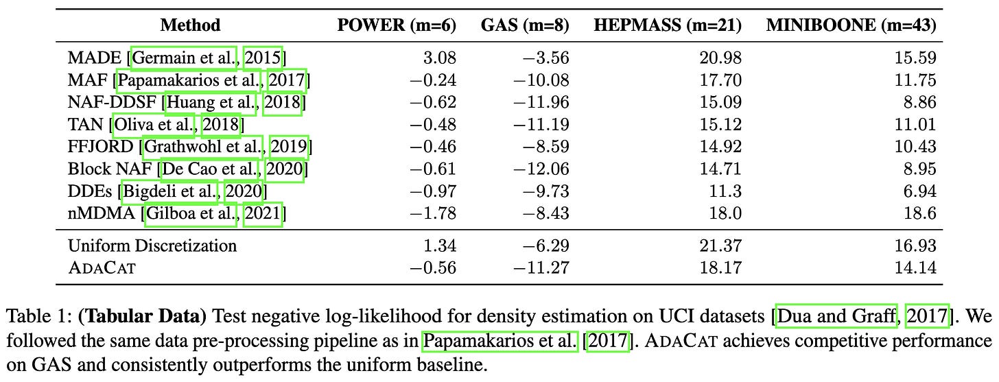
AdaCat: Adaptive Categorical Discretization for Autoregressive Models
They decompose the joint distribution of multiple scalar variables into a sequence of conditional distributions using a deep autoregressive model, and then use a differentiable and heuristic alternative to piecewise constant approximation to construct quantization bins for the conditional PDF.
Seems to work decently for various density estimation and other tasks.
Few-shot Learning with Retrieval Augmented Language Models
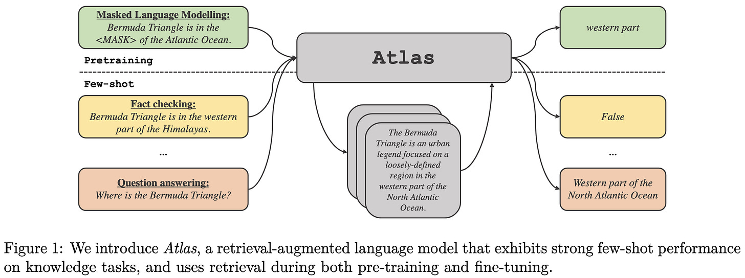
New SotA on NaturalQuestions, TriviaQA, FEVER, and 5 KILT tasks with an 11B-parameter retrieval-augment model. These results include beating models like PaLM that used up to 50x more pretraining compute.
To do this, they use a T5 augmented with a Contriever that embeds queries and documents in the same space. They run each retrieved document through the T5 encoder separately, concatenate all their encodings, and pass the result to the decoder.
During pretraining, they add a loss for the retriever to that tells it to retrieve documents useful for the pretraining task. They investigate several possible losses, such minimizing the difference between a document’s retrieval probability and its average attention weight in the main model.
They find that certain losses work better than others, and that jointly training the retriever definitely helps.
They also test something a lot of us have been curious about: the value of swapping out the retrieval database to adapt to changing facts. Using a dataset of Google searches from 2018, they found that using a 2018 Wikipedia dump gave the best results.
Overall, this is a a thorough paper with a lot of convincing results and interesting ablations. Further evidence that adding retrieval can be a huge lift.


