2022-8-21 arXiv roundup: RecSys scaling, PatchDropout, LLM.int8()
This newsletter made possible by MosaicML.
PatchDropout: Economizing Vision Transformers Using Patch Dropout
When training DeiT or Swin transformers, you can just drop half the input patches at random and it’s totally fine.
If you want to go crazy, you can drop even more than that for a larger speedup at the cost of accuracy.
This time vs accuracy tradeoff is so good that you’re usually better off training a larger model with more patch dropping than a smaller model with no patch dropping.
Similarly, you’re often better off using 4x as many input pixels but dropping 75% of the patches (compare the first and third entries in each block of rows).
Dropping half the patches can even give you increased accuracy, probably because it acts as a Cutout-like form of regularization.
You need to use the full image at inference time though, or you’ll likely get accuracy loss.
I really like this paper. It proposes a simple idea that works well in practice and has a thorough, easy-to-follow evaluation.
Method-wise, it reminds me a lot of Learning to Merge Tokens in Vision Transformers, where they instead add a layer of learned queries that reduces the input to a fixed number of patches. This number is a complicated function of model size, input resolution, and sample count, by which I mean, literally always eight, independent of any of those factors.
This paper makes we wonder how well we could do with intelligent patch selection schemes, especially at inference time. I’m also curious how this compares to progressive resizing, which was a big help in our winning MLPerf submission.
Understanding Scaling Laws for Recommendation Models
Studies scaling laws for click-through rate prediction models—i.e., the main recommender systems that make all the $$ in digital advertising.
tl;dr: “We show that parameter scaling is out of steam for the model architecture under study, and until a higher-performing model architecture emerges, data scaling is the path forward.”
It’s kind of hard to keep track of what’s going on here because they’re simultaneously looking at total training compute, dataset size, total parameter count, and four different ways of scaling up parameter count: increasing the number of embeddings (V), embedding dimensionality (H), upper-level MLP widths (M), and overall non-embedding-parameter widths (O).
The main takeaway in most plots is that individual curves (corresponding to increasing parameter count) are flat, while successive curves (corresponding to more data) have decreasing loss.
Also, they find that how you scale up your model’s parameter count (e.g., making the embeddings bigger vs making the MLP bigger) doesn’t affect data scaling much.
But that doesn’t mean you should ignore how to scale up the model entirely. They run numerous experiments here, and find some pretty clear patterns. This finding that how you scale the model matters stands in contrast to earlier NLP scaling work, which argued that “model shape” wasn’t important.
There isn’t a single answer for how you should scale up your recommender model’s parameters though. Instead, it depends on how much compute and data you have.
Perhaps the least surprising result is that the data scaling exponent for the train loss is much better than that of the test loss. Though it is interesting that this shows up in the exponent rather than just, e.g., the leading constant or irreducible loss.
What I’d love to know here is how exactly they got these curves. In particular, were they doing single-epoch training? It seems like they were since they don’t distinguish between data and optimization steps. And if so, are the points on the curves individual training runs, or just intermediate losses from one run? Using the latter is what caused Kaplan et al. to underestimate the data scaling exponent, so there’s some chance that data is even more important than this paper suggests.
But overall, this is exceptionally thorough and interesting work, and I’m sure it will make Google and Meta an enormous amount of money.
LLM.int8(): 8-bit Matrix Multiplication for Transformers at Scale
They quantize transformer weights to 8 bits so that they fit in smaller GPUs for inference.
From a quantization perspective, there doesn’t seem to be anything here that wasn’t in FBGEMM in 2018. They partition tensors into inliers (small norm) and outliers (large norm), and do int8 and f16 matmuls for these two groups, respectively. No disrespect over the limited “novelty”—this just means they went with what worked the best rather than what would impress reviewers.
What’s much more novel and interesting here is the exploration of outlier activations and how they change as a function of model size.
First, one helpful finding is that huge activations are concentrated within particular feature dimensions. For one 13B param model, they found that 7 features accounted for *all* of the outliers.
Along the same lines, which features have outliers is consistent across layers. I suppose this makes sense given the skip connections driving features to have consistent “meaning” across layers?
Third, outliers happen more consistently as model size increases and perplexity decreases. Although it’s a vague trend that’s hard to fit a curve to, rather than a clear scaling law or regime change.
Fourth, outliers increase in magnitude and frequency as model size increases / perplexity decreases, seemingly at a superlinear rate.
At present, their approach is around 20% slower than f16 inference. But this mostly seems to be a matter of implementation details, and they’re working on it.
Also wanna give them props for this: “to make sure that the observed phenomena are not due to bugs in software, we evaluate transformers that were trained in three different software frameworks.” Controlling for library differences is really important and I wish more people did this.
If you find this work interesting, I’d definitely recommend reading their blog post for more details.
Adan: Adaptive Nesterov Momentum Algorithm for Faster Optimizing Deep Models
Another optimizer paper attempting to descend through a crowded valley to beat Adam.
Their update equation is fairly straightforward, and complements the gradient momentum term with a difference-of-gradients momentum term.
It does have an extra hyperparameter compared to Adam (β3), but they hardcode it to 0.08 in all their experiments, so it’s apparently not important to tune.
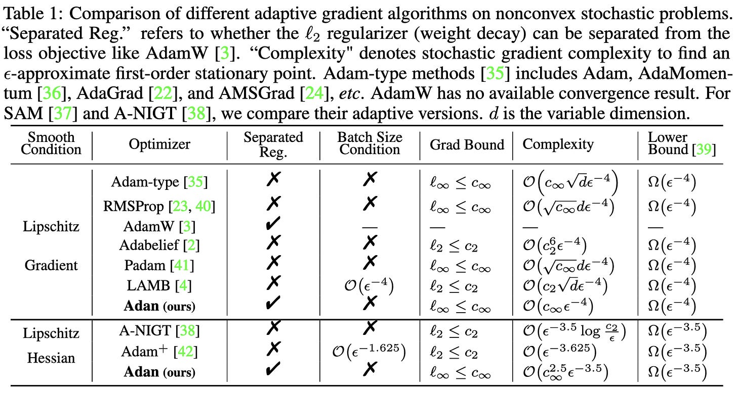
They have good theoretical guarantees, essentially attaining known lower bounds.
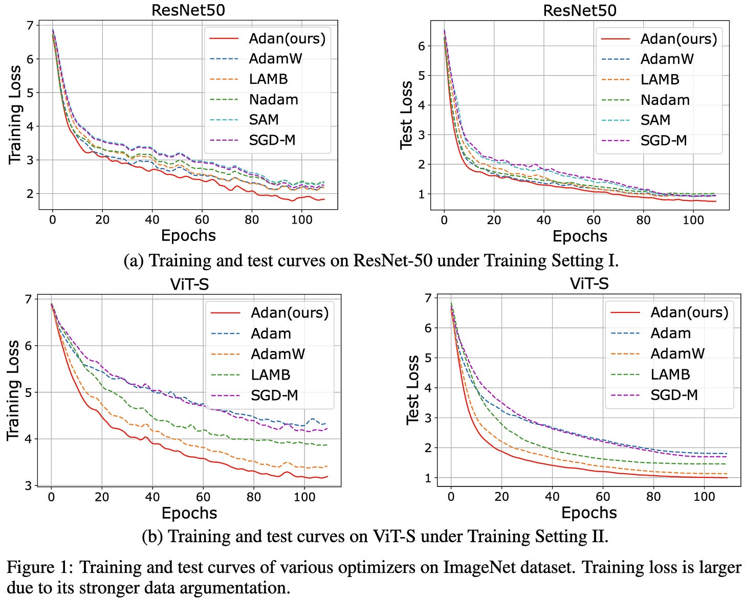
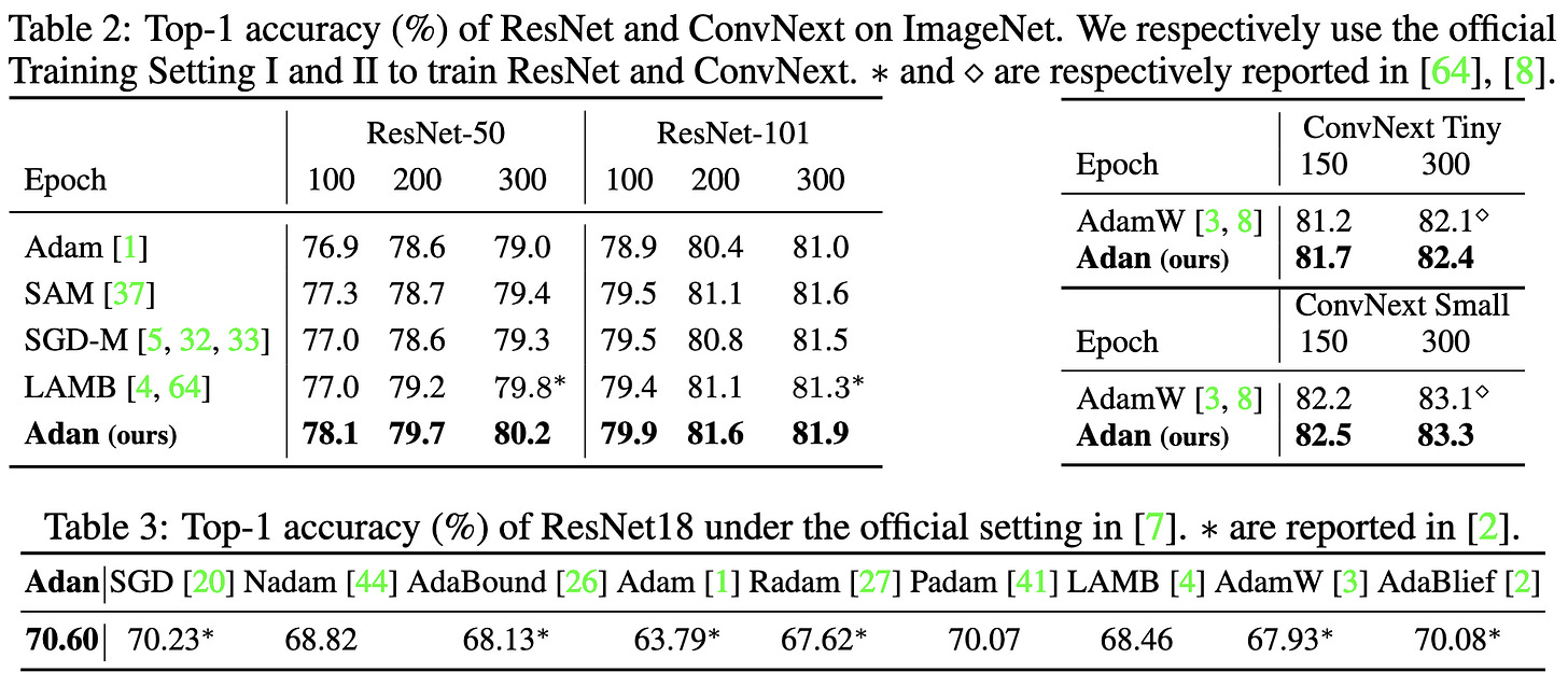
Most importantly, they consistently beat other optimizers across a variety of vision, language, and RL tasks.
I always assume papers introducing new Adam-like optimizers are just some mix of grad student descent, subtly messing up the baselines, unfair hparam tuning, etc. But this is so many accuracy lifts, so consistently, across so many tasks that I could believe the improvements are real here.
An Algorithm-Hardware Co-Optimized Framework for Accelerating N:M Sparse Transformers
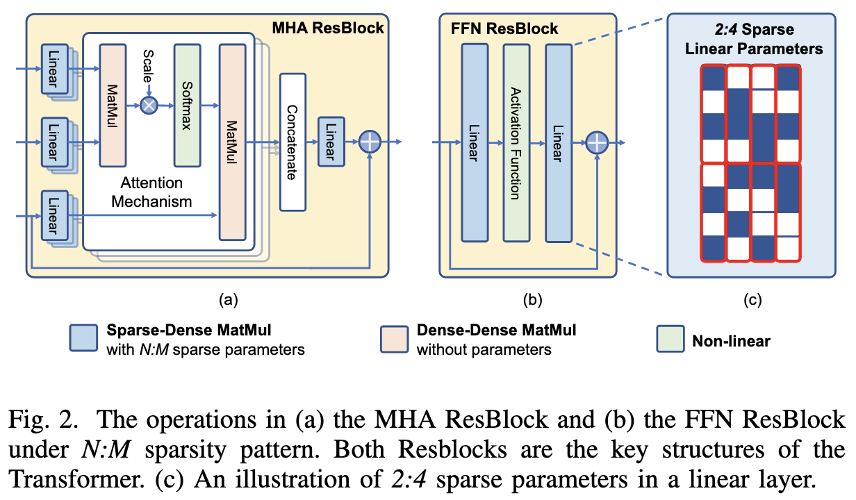
They apply Ampere-friendly N:M sparse pruning to various models and also propose a hardware acceleration approach.
Here’s where they add the sparsity:
They do iterative magnitude pruning on the network (with an N:M sparsity constraint) to get their sparse network.
Their method (IDP) works better than some baselines, but boy does BERT lose accuracy fast as you prune it.
Conviformers: Convolutionally guided Vision Transformer
Couldn’t tell much from their main results, but they propose an interesting preprocessing step. Ignoring the dataset-specific cropping part, they propose to pad the shorter side with mode “reflect” rather than using zeroes, cropping, or rescaling.
This strikes me as probably not a great idea for landscape images, where reflection means vflipping an image; but I could see this being a cheap way to also train on an hflipped copy for portrait mode images. Since hflipping is one of the most helpful data augmentations for natural images, this fused pad + hflip could be valuable.
Empirically, this preprocessing helps a little bit on their plant dataset:
Zeus: Understanding and Optimizing GPU Energy Consumption of DNN Training
By optimizing the batch size and GPU power limit, you can improve the tradeoff between time-to-train and energy-to-train.
And it can be a big improvement. Here they cut energy-to-train by a third with no slowdown by nailing the batch size and power limit:
So the question is how to optimize these two quantities for a given training job. The power limit is easy to optimize. It doesn’t affect the computation, so it’s just a matter of microbenchmarking during training.
Getting the batch size right is tricker. One approach is to just launch an hparam sweep to figure out what batch size trains in the least wall time. But that adds a lot of extra work.
Instead, they assume you’re running a recurring training job and frame this as a multi-armed bandit problem. For each training run, they use Thompson sampling to generate a batch size.
They impose a Gaussian form on the distribution of time-to-accuracies given a batch size. This method is simple and makes it easy to deal with distribution shift by throwing away or downweighting old observations.
They evaluate their approach on a variety of reasonable tasks, although arguably with low target metrics (e.g., 65% for ResNet-50 on ImageNet).
Their method consistently reduces energy usage while keeping training time about the same.
As you might expect, Thompson sampling does better than brute force search.
The main limitation I see overall is the difficulty of translating power consumption to environmental or financial impact. Most of the carbon footprint of computing comes from manufacturing the devices, not running them.
It’s also hard to save money by reducing power consumption; this is partly because energy cost is small relative to hardware cost, and partly because datacenters usually charge you for peak power required, not actual power consumed.
But for, e.g., a FANG company that owns its own datacenters and fills them with bulk-discounted hardware, I could see the energy savings being super valuable.
Overall, it’s cool work tackling an important problem in a principled way. I especially appreciate how they went with Thompson sampling rather than, e.g., some crazy RL scheme that would complicate their method and evaluation.


