
2022-10-9 arXiv roundup: The death of depth?, Vision pretraining throwdown, Parameter-efficient MoE

Oh man, we got some good stuff this week.
But first, quick thanks to MosaicML for making this newsletter possible, as well as @andrew_n_carr, @dpaleka, @Muhtasham9, @code_star @abhi_venigalla, and all the other nice people on Twitter who randomly recommended this newsletter this week. I normally just hit “publish” and don’t hear anything back, so it means a lot when people say they like it.
Wide Attention Is The Way Forward For Transformers
Instead of using an L-layer transformer with H attention heads, they use a 1-layer transformer with L*H attention heads. Turns out this is just as good or better.

More precisely, on four sequence classification tasks, they find that wider models are at least as good as deeper ones on average. And this result doesn’t just hold with vanilla self-attention, but across a variety of different attention mechanisms.

This result also holds for various points on the spectrum between the original deep models and the wide-only models. I.e., L/k layers with kH heads per layer for any k ≥ 1.


The best part is that the wider models are way faster. This is because they keep the amount of computation in the attention mechanism constant, but have only one FFN. Since FFNs are usually most of the compute, this gets them a >2x savings.

They also argue that shallow models with many attention heads can be more interpretable, with high attention weights corresponding to important tokens for the prediction.

However, for vision tasks, just going wide doesn’t seem to work. They attribute this to the importance of spatial information + having some sort of pooling.

Lastly, they try out using different attention mechanisms for different heads. This tends to work better than the average accuracy across different attention mechanisms, but not as well as choosing the best attention mechanism for that task.

Overall, this proposed architecture change is one of the largest accuracy-preserving speedups I’ve ever seen. I’m not positive accuracy preservation will hold for billion-parameter models, where the FFNs are almost all of the compute. But even if we can only, say, double the widths of the attentions and halve the depths, that’s still a big win. Plus, less depth means fewer numerical issues, making formats like fp8 more appealing.
Also, it's kind of embarrassing that it took us as a field 5 years to run this ablation.1 There's a lesson here about thinking from first principles and never taking "standard" practices for granted.
MLPInit: Embarrassingly Simple GNN Training Acceleration with MLP Initialization
They observe that:
1) You can treat a message-passing-based graph neural net as an MLP, just rolling the adjacency matrix into the weights.

2) If you ignore the adjacency matrix and directly train an MLP on each node’s features, you initially get more accuracy per epoch and per unit time.
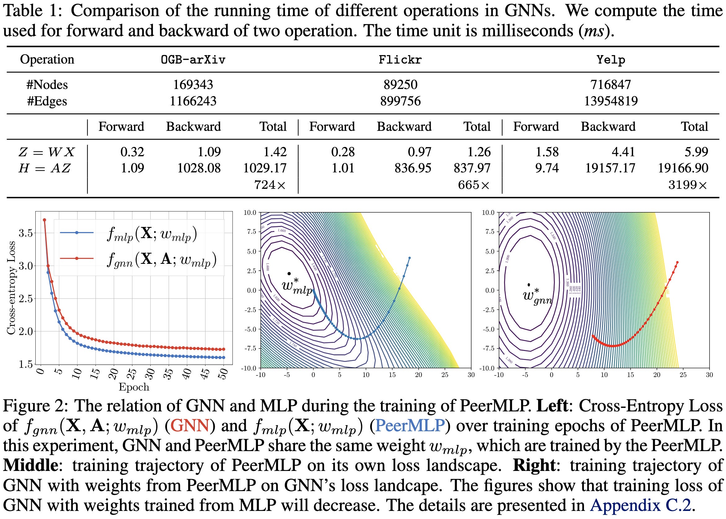
3) You can use the resulting MLP’s weights to initialize your GCN, getting you way more accuracy in less training time than a randomly-initialized GCN. I.e., after training the MLP, finetune with the adjacency matrix present.

This is pretty elegant, and makes we wonder whether there are similar initialization schemes for other classes of models—that is, pretrained weights not from the same architecture, but from a different weight-compatible architecture that trains way faster.
Self-Stabilization: The Implicit Bias of Gradient Descent at the Edge of Stability
They show why, under reasonable assumptions, gradient descent tends to hover at the edge of stability. Recall that the edge of stability means that the operator norm of the local Hessian is 2/η, where η is the learning rate. This 2/η is the most curvature one can have without the iterates diverging.

To show this, they consider just the movement of the iterates in two directions: the direction of the largest eigenvector of the Hessian (the sharpest / most unstable axis), and the direction of greatest sharpness change.
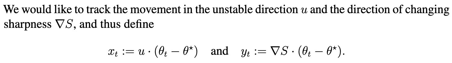
Under the assumption that this direction of increasing sharpness points at least partially in the same direction as the negative gradient, they derive a negative feedback loop keeping gradient descent right at the edge of stability.

What happens is that, when you enter an excessively sharp part of the landscape and your iterates start diverging, the third-order term of the local Taylor expansion starts to dominate. And this term moves you in the direction of decreasing sharpness.

So the cycle is:
Follow the gradient, which increases sharpness (by assumption/empiricism)
The increased sharpness makes you start to diverge
As you diverge, the 3rd-order term takes over and moves you in the direction of decreased sharpness.
This apparently lines up super well with observed training dynamics, at least on small-ish experiments:

Pretty cool work. I’d need to derive the 3rd-order gradient to really grok it, but it’s explained well and seems to predict reality. Still doesn’t explain why the gradient direction and sharpness direction are negatively correlated though—maybe subquadratic loss landscapes?
Neural Graphical Models
So let’s say you have a known graph structure for your variables and you want to learn to estimate each variable given its neighbors. Just construct an autoencoder with carefully chosen edges that reflect your (in)dependencies.

Where Should I Spend My FLOPS? Efficiency Evaluations of Visual Pre-training Methods
They systematically try different pretraining methods for different downstream vision tasks.

CLIP pretraining often works the best for a fixed budget of pretraining FLOPs (below) and time (above). Supervised classification is the second best, followed by masked autoencoding. Also, you need to use a larger model when throwing more FLOPs at pretraining.

Regular old ImageNet-1k is often the best pretraining dataset. This might be because it tends to have centered images of objects with less-bad labels than anything else.

The ordering for CLIP, supervised, and MAE isn’t always consistent. For COCO detection after pretraining on a huge image+caption dataset, MAE beats the other two.
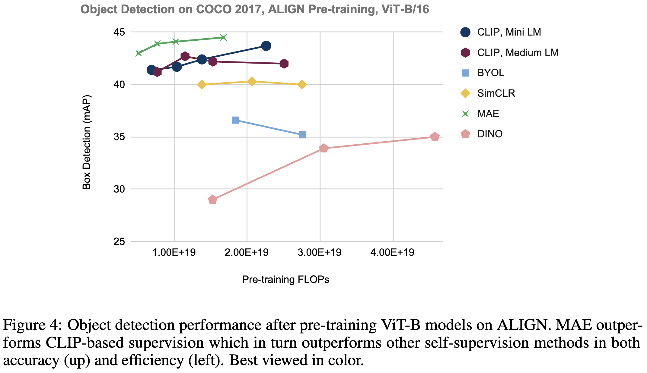
But if you swap out the pretraining dataset, CLIP becomes better.

They also include results for per-step costs of each method. DINO is crazy expensive and MAE can be really cheap. Supervised and CLIP training are in the middle.

I really like this paper. Systematic comparisons of different methods under controlled conditions are extremely valuable—especially when there’s no “proposed” method to bias the authors.
Since MAE is coupled to vision transformers, I’ll probably use CLIP as my go-to pretraining method. Although there are so many vision SSL methods out there that I could imagine DetCon or something else actually being the best.
ByteTransformer: A High-Performance Transformer Boosted for Variable-Length Inputs
No, not a transformer that operates directly on bytes—a transformer from ByteDance.
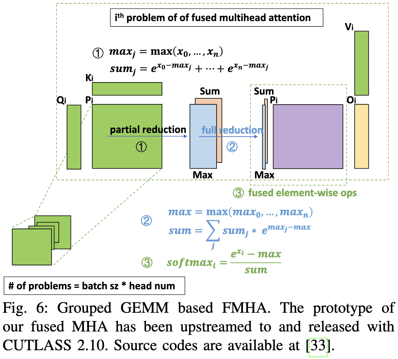
Basically they propose an efficient attention implementation similar to FlashAttention. But instead of just having operator fusions, they also use grouped GEMMs to handle variable-length sequences without padding. A grouped GEMM is like a batch GEMM but the individual matrix products can have different matrix sizes.

They also fuse layernorms, bias addition, and GELUs. All of these optimizations together yield around a 2x speedup, depending on the sequence length. Though the 2x would go down if the sequences were closer to uniform length (their benchmark makes them 60% of the padded length on average).

End-to-end, they beat alternative attention block implementations by a lot. Though, probably due to being concurrent work, they don’t compare to FlashAttention, the current SotA.

The other noteworthy aspect is that their fused MHA apparently got upstreamed into CUTLASS, which is both a strong quality signal and suggests you might actually be able to use it.
Finally, here are some profiling results they had for BERT-Base inference on an A100 (batch size not stated). At this model scale, vanilla PyTorch attention takes up 22% of the time for sequence length 256, but 49% of the time for sequence length 1024.

Transformers Implement First-Order Logic with Majority Quantifiers
They show that many neural nets, including transformers, can be expressed in FO(M)—i.e. first-order logic that has a “majority” quantifier in addition to “there exists” and “for all.”

You’ll have to really sit down with this paper to understand it, but the implications are super cool. Basically, formal logic is both way easier to interpret and way easier to prove guarantees about than giant blobs of tensor ops. Which suggests that, rather than heuristic approaches that we hope will get models to do what we want, we might be able to formally guarantee that models will do what we want.
Of course, formal verification is hard even when your whole language is designed for it. But still, this paper makes me more bullish on formally verifying neural nets a possibility.
Revisiting Structured Dropout
They drop out activations in proportion to their absolute value. When dropping out one activation, they also drop out activations in a square around it.

Seems to do about as well as other dropout variants, and consistently helps vs the baseline training setup a little bit. The baseline BatchDropBlock (tying what gets dropped across the whole batch) often hurts accuracy.


Mostly they have two claims about how to do dropout that I find interesting. First, they provide some evidence that linearly ramping up the drop probability from 0 to some constant helps, consistent with previous work.

Second, based on BatchDropBlock doing terribly on language tasks, they claim that dropping heads independently across different samples in a batch is important. This is unfortunate from a speed perspective, but sometimes that’s how it goes.
Language Models are Multilingual Chain-of-Thought Reasoners
Introduces the Multilingual Grade School Math (MGSM) benchmark, which consists of the same math problems translated into various languages. Models are a little better at this in higher-resource languages, but still pretty good even in low-resource languages. Bigger models do better.

Are All Losses Created Equal: A Neural Collapse Perspective
Common losses like cross-entropy, focal loss, cross-entropy with label smoothing, and mean squared error eventually drive all samples from a given class to have the same representation at the last layer. Also, the average representations of the different classes all have equal magnitudes and point in (equally) opposite directions as much as possible given the embedding dimensionality.
Basically, they do what you’d expect if you think about what would yield the highest softmax probability for the correct class subject to norm constraints.
This collapse phenomenon has been observed before, but this paper explores the extent to which different common losses avoid it.
tl;dr, they don’t avoid it, and are all about equally susceptible.
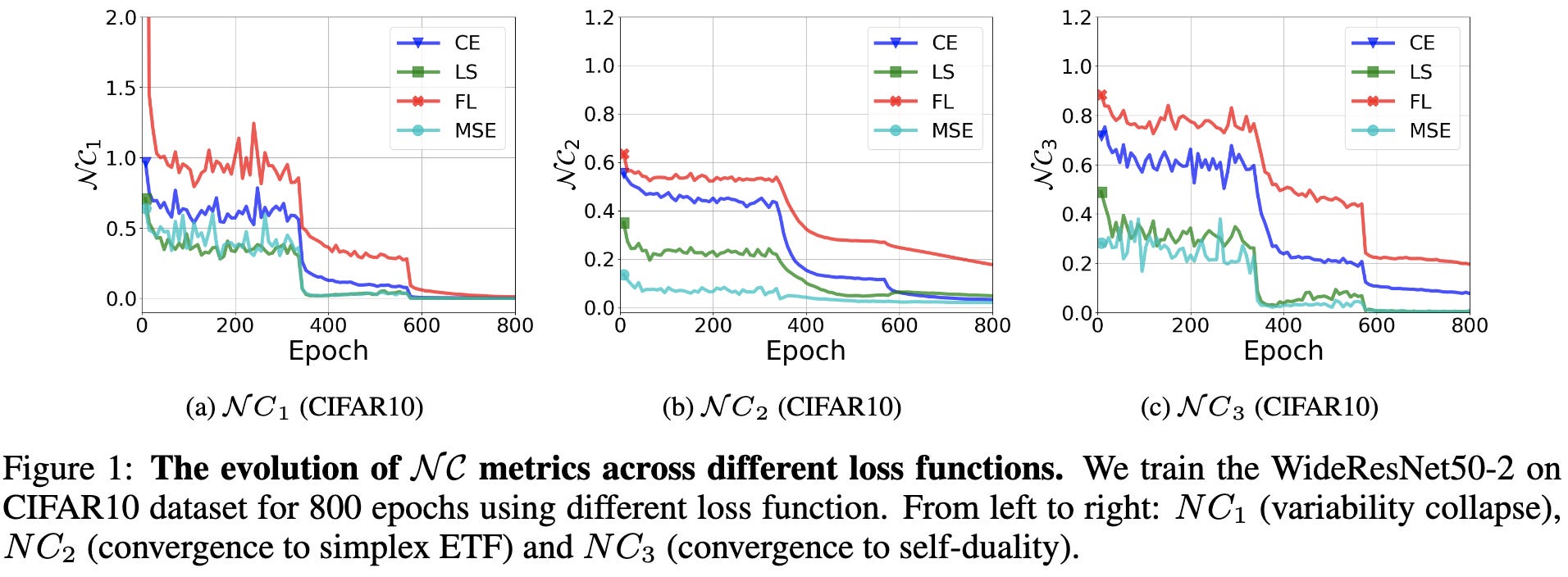
Imagen Video: High Definition Video Generation with Diffusion Models
Google extended Imagen to do text-to-video. Their example videos are awesome.
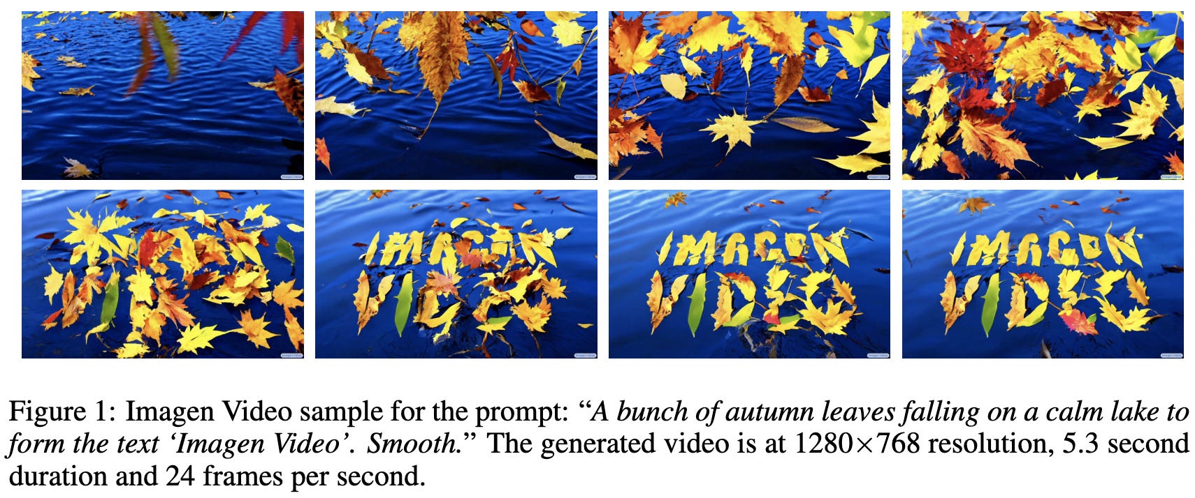
To do this, they use a Video U-Net along with a cascade of diffusion-based super-resolution models to upsample in both pixel space and time. The final resolution and frame count are fixed.

The Video U-Net does convolutions and attention separately in space and time.
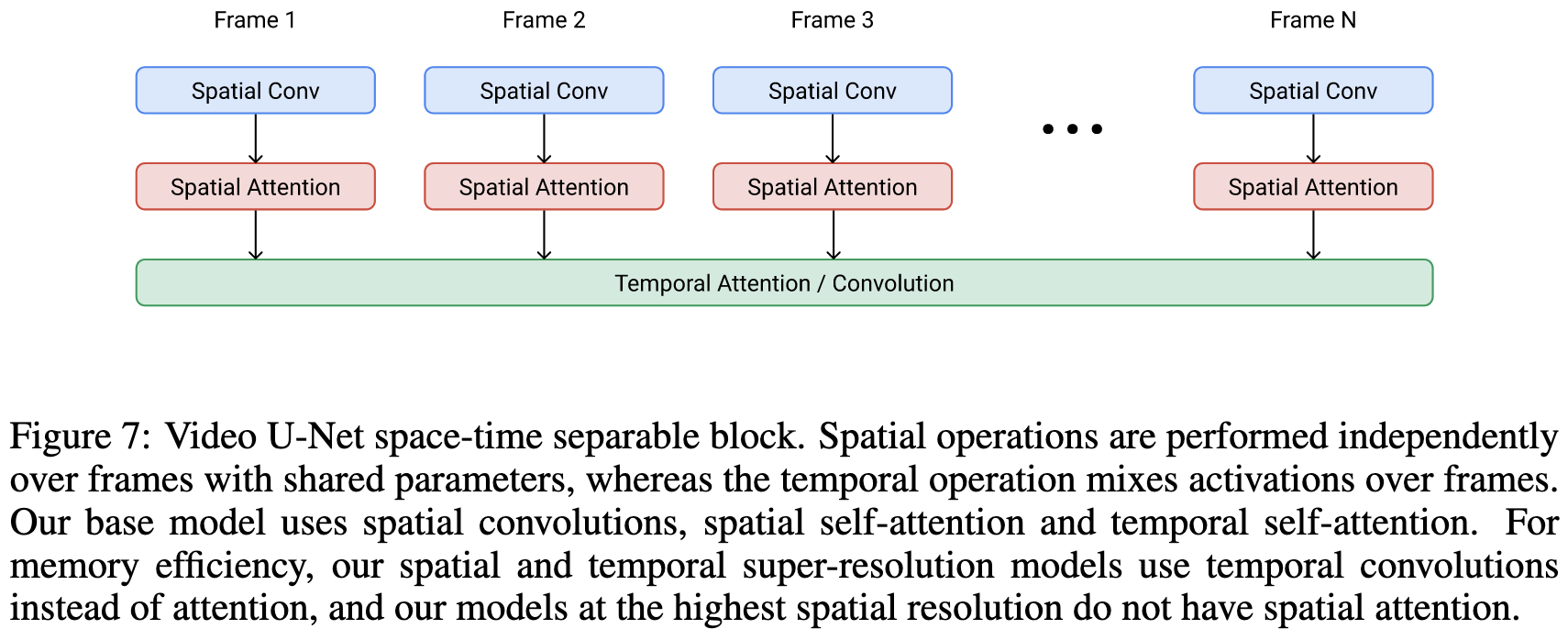
It took a lot of specific design choices to get it working well—e.g., v-prediction, conditioning augmentation, classifier-free guidance, and joint image-video training (treating images as single-frame videos), among others. They also use progressive distillation to get the inference latency of their diffusion models down.
The Dynamics of Sharpness-Aware Minimization: Bouncing Across Ravines and Drifting Towards Wide Minima
With a quadratic objective, SAM causes the iterates to oscillate around the minimum along the axis of greatest curvature and never converge.
With non-constant Hessian though, SAM has a 2nd-order term that causes its oscillations to descend in the direction of decreasing Hessian spectral norm (i.e., sharpness).
This makes me wonder whether SAM just finds flatter minima because of this 2nd-order term, if it tends to end up in entirely different basins of the loss landscape, or both. Also, if it oscillates even in the quadratic case (while SGD wouldn’t), should we be turning SAM off late in training?
Omnigrok: Grokking Beyond Algorithmic Data
It's common for your training loss to decrease monotonically with weight norm, while your test loss goes down and then comes back up.2 They argue that grokking, rather than being some weird quirk of algorithmic tasks, is just what happens when your weights start off too large, rather than too small.

When your initial weights are too large and you barely have any regularization to shrink them, it takes a ton of time for the weight norms to get small enough for the model to generalize.

In fact, you can even induce grokking through large initializations with small regularization.

Their explanation for why grokking tends to happen on algorithmic datasets is that these tasks are more all-or-nothing as far as whether your representation is good enough to get the right answer—similar to what we see with exact match vs multiple choice questions for language models.
Besides shedding light on grokking, this makes me way more scared of using too large an initialization, as opposed to too small an initialization.
Scaling Laws for a Multi-Agent Reinforcement Learning Model
They got decent power law fits for Connect Four and Pentago agents.
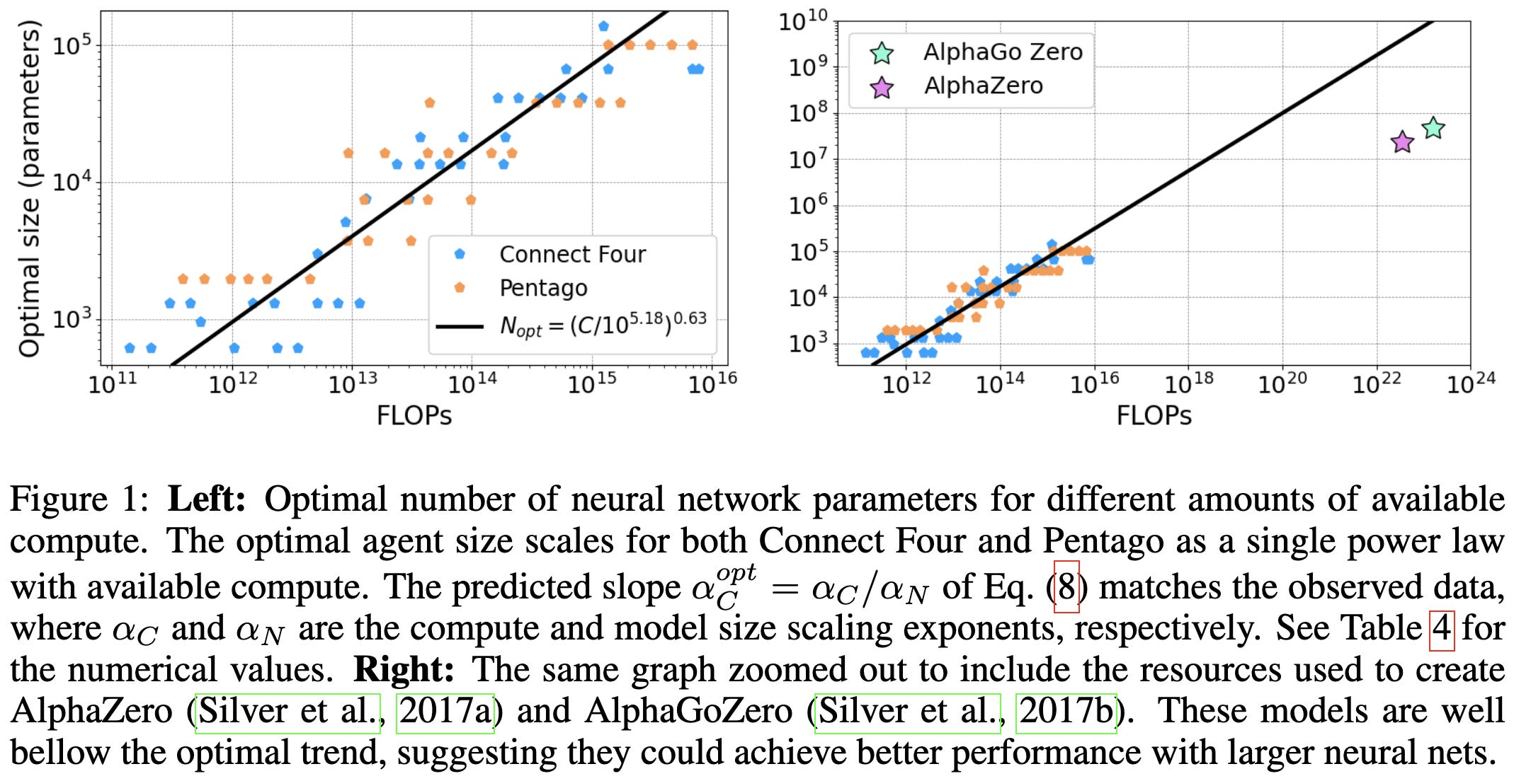
The exponents for the two games are surprisingly similar.

The main subtlety here is that Elo is a logarithmic measure of player skill, so power laws look like logarithmic scaling with respect to the x variable.
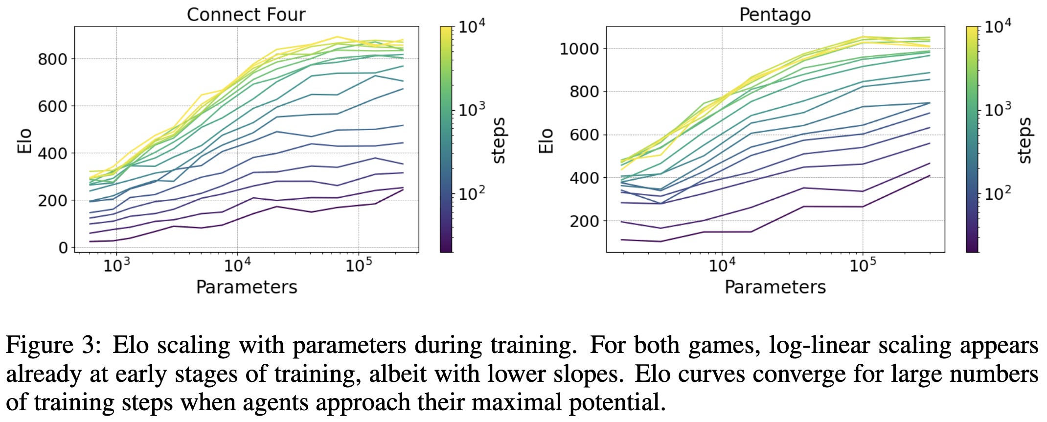
As an aside, they remark that they managed to observe these scaling laws (in an earlier study) in small-scale experiments with just a 4-core CPU, and suggest that this bodes well for budget-constrained research groups.
Limitations of neural network training due to numerical instability of backpropagation
We’ve talked before about how ReLU networks are locally linear within each of many tiny regions of the input space.
This paper does analysis implying that real deep networks don’t have nearly as many regions as what’s theoretically possible. In fact, rather than having a number of regions exponential with depth, they don’t even manage to get superlinear. This is largely a consequence of floating point errors.
In experiments on toy networks, they confirm this result. The number of unique sets of nonzero activations (right subplots) is tiny compared to what it could be.

But here’s what I thought was most interesting. In the next experiment, they still try to learn a quadratic function, but initialize their network to compute a quadratic function from the outset. In the upper left plot, they get exponential decay in loss with respect to iterations. Not a power law. Exponential. I’ve never seen this before, and it would amazing if we could obtain this improved scaling on real problems.
The caveat here is that, with four more layers, they jump straight to the lowest error possible (lower left). So maybe this exponential decay is only attainable for trivial problems.
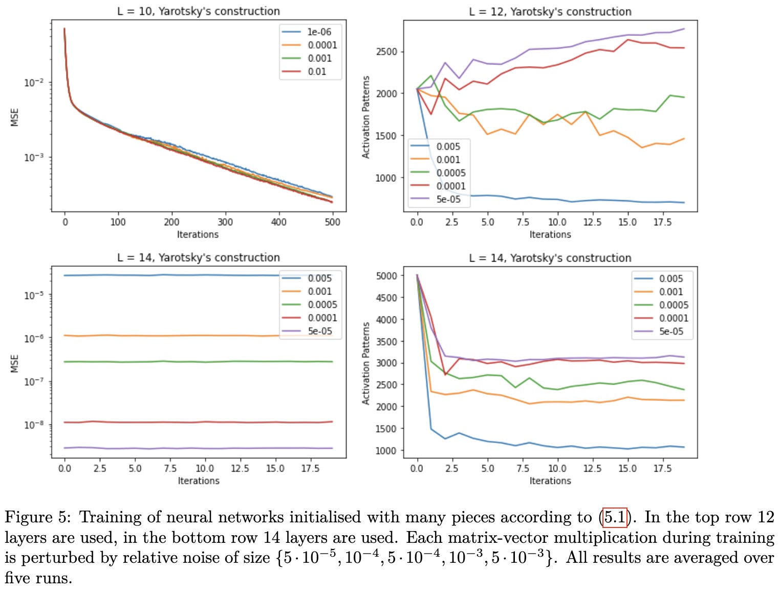
So this paper both made me hopeful that better-than-power-law scaling might be possible in some cases, but also a more pessimistic about low-precision training. I’d always thought of numerical issues as mostly being a problem for computing gradients with respect to inputs—but their results suggest that low-precision in forward can limit model capacity.
SimPer: Simple Self-Supervised Learning of Periodic Targets
They design an SSL algorithm for periodic data, and show that you should definitely use such an algorithm if you know your data is periodic.

By “definitely,” I mean you can get huge error reductions consistently across a variety of datasets that have this structure.

Makes me wonder what other inductive biases we should be baking into our SSL algorithms.
Go Wider Instead of Deeper
There are a bunch of interesting results in this paper.
Their method is just to add mixture of experts to all the FFNs in your transformer, but tie all the non-norm parameters across all the blocks. This gets you parameter count increase (nearly) proportional to your expert count, but a parameter count decrease proportional to your number of transformer blocks.

The first result is that, like most MoE work, they get significant accuracy gains. What’s surprising is that they get these gains not with way more parameters, but with fewer.
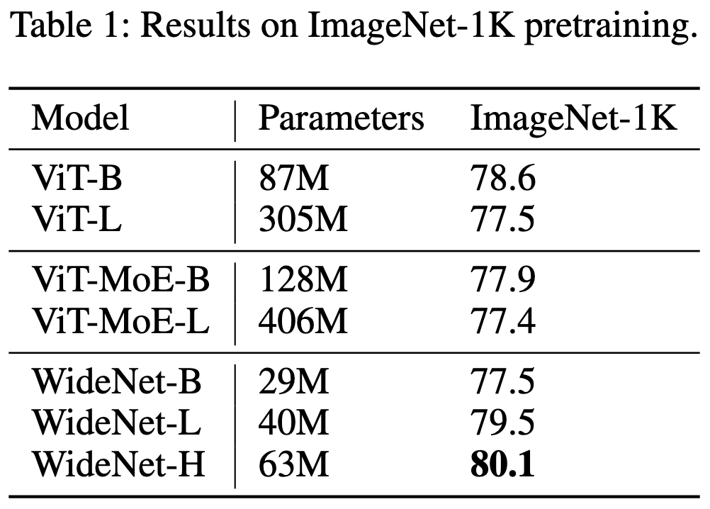
This holds for both image classification and some GLUE tasks.

The story is a bit less clear if you control for training time. They do a little better in this case, but it’s much less improvement than we usually see in MoE papers.

So they seem to save model size more than they save time—though I could imagine just not sharing params across all the layers might let them tune this to a better operating point.
But here’s the most interesting result: for ViT-L, sharing parameters increases ImageNet accuracy. This isn’t true for ViT-B and they don’t tell us if it’s true for ViT-H, but this still flies in the face of normal neural net scaling.
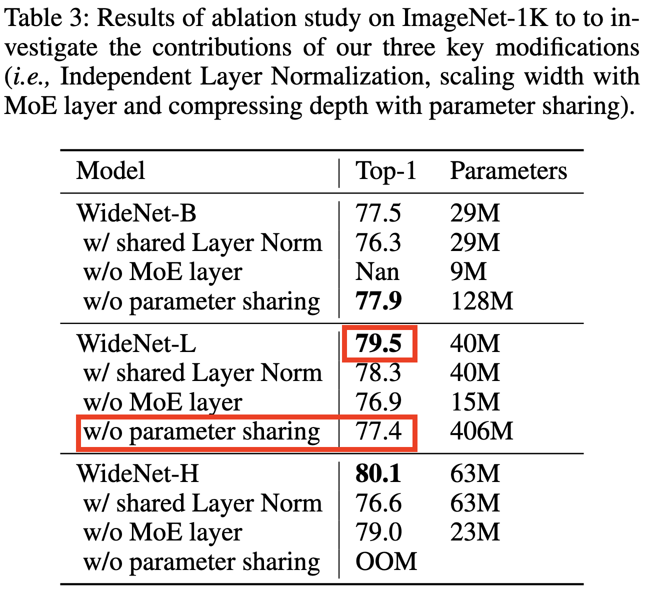
They explain this by observing that cranking up the expert count with regular MoE tends to overfit on ImageNet, since it’s not that many unique samples. They also conjecture that this is a product of each expert not getting to see as many samples.

The latter conjecture—the importance of having enough samples to support your expert count—is consistent with my experience. I tried running some simple MoE stuff on CIFAR-10 and CIFAR-100 (which only have 50k training samples), and let me tell you, it was like trying to squeeze accuracy out of a rock.3
So overall, I’m not sure parameter sharing + MoE is usually the way to go, but there does appear to be a regime wherein sharing parameters with MoE is strictly better than not sharing them. And, more generally, I’d conjecture that there’s some optimal amount of sharing for a given task/model.
Really cool results that provide both accuracy gains and insights into MoE models.
I wanted to run an experiment like this for a long time but never got around to it. That totally counts, right?
Also, they reference a claim in some of Andrew Ng’s lecture notes (link broken) that double descent doesn’t violate the U-shape of the test loss. The way to reconcile this is to look at the norm of the parameters, rather than the count. I.e., double descent is when models with more parameters end up with smaller parameter norms.
I do wonder though whether ImageNet not being enough data in their experiments is partially an artifact of using plain vision transformers, which tend to be much less data-efficient than CNNs.
The Wide Attention paper is misleading. They only perform experiments on the tasks where even a bag-of-words model gets good performance. I got much worse performance when I tried this on other tasks.