2024-4-14 arXiv roundup: backlog highlights part 2
Bunch of interesting stuff this week.
Before we jump in, one quick clarification from last week: I mentioned how it was an interesting marketing lesson from DBRX development how we spent a bunch of time adding to MegaBlocks but then people ended up associating it with Mistral because they released an MoE first. A couple people said this part was “super spicy” (maybe because of the phrasing of the tweet I screenshotted?) so just to be explicit: I see this purely as a case study in marketing + open source, and no one at Databricks has anything against Mistral at all. We have a ton of respect for them and their models, and I hope they get to succeed as a startup too.
Anyway…
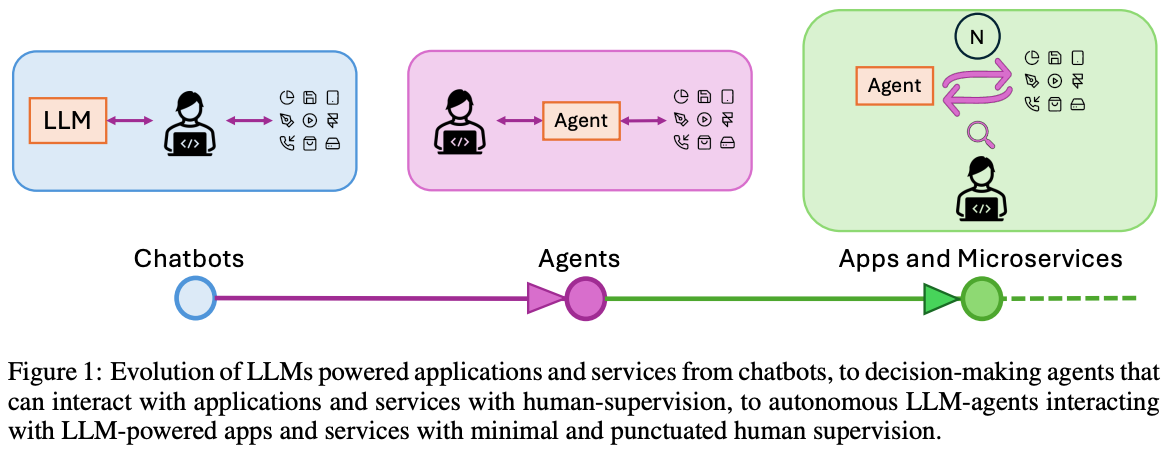
GoEX: Perspectives and Designs Towards a Runtime for Autonomous LLM Applications
This is one of those rare papers that really changed my thinking about where we’re headed.
I’ve thought for a long time about how LLM-generated code would need to be sandboxed, and how you probably want to sanitize the inputs in various ways, and how you might want to postprocess or constrain the outputs to do something like guarantee that you’re getting valid JSON.
This paper points out that what we really want is not a bunch of separate pieces, but a cohesive LLM Runtime that enforces certain properties, even in the presence of an untrusted LLM agent. Some example properties include:
Ensuring your LLM agent’s actions are “reversible,” meaning that you can always undo them if you don’t like them.
If you can’t get full reversibility, enforcing “damage confinement,” so that the persistent side-effects are well-understood and the rest of the system can work around them. E.g., you can’t un-send an email, but you might have a whitelist of recipients and MIME types.
Ensuring that cryptographic secrets don’t get shared with third-party LLM APIs.
Sandboxing code execution (think VMs, Docker, WASM, intercepting syscalls, limiting dependencies, etc).
To achieve these properties, they lean on a lot of ideas from classic data systems, like ACID transactions and commits.
While the paper reads like a position paper on LLM agents initially, you realize halfway through that this is hardcore systems research. Like, look at all these different runtime components they built just to safely hit a REST API:
Similarly, they end up with some interesting design tradeoffs around damage control/reversibility. The easy case is if you can lean on a database to just handle undo operations for you. The harder case is if the actions are too complex to cleanly undo, and you have to snapshot different versions of your system state and restore them.
I’m excited about this for a few reasons.
First, it’s just much cleaner thinking about what we need in order to make agents safe to deploy. I’d previously only thought about a hodgepodge of hammers and nails, but formulating this as “We need to design an LLM runtime with a particular threat model that guarantees particular properties” is much clearer.
The second is that this clean formulation means the field will pick up on this idea and make real progress. We’ll see systems researchers for the next 5+ years gradually tightening the guarantees, reducing the overheads, expanding the functionality, etc. We’ll see open source LLM runtimes, with auditable security properties. We’ll see vendor solutions that integrate with containers and/or hypervisors. We’ll see public REST and GraphQL APIs start to add reversibility features to facilitate calls from agents. And more.
The last reason is that I see this as a promising attack on AI doom scenarios. For a long time, this literature has focused on extremely high-level failure modes (e.g., humans being disempowered as we grow dependent on AI) and properties of agents (e.g., being aligned with human values). I feel like this paper has “compiled” many abstract concerns down to the level of verifiable system properties—like, if we can “undo” an agent’s actions, it probably can’t kill us all.
On a more meta level, it also reinforces my conviction in the following maxim:
Never solve with machine learning that which can be solved with regular code.1
For example, people spent decades trying to come up with some algorithmic alternative to backpropagation, in part to avoid the (biologically implausible) storage of activations and synchronous updates. But it turns out we can just devise systems improvements like sharded data parallelism, pipeline parallelism, etc, that make these downsides fine in practice. It’s much easier to make working algorithms fast than to find fast algorithms that work.
In the case of this paper and AI doom, I feel like we’ve spent decades thinking about high-level problems like specifying human values and “target loading” and detecting “deceptive alignment,” and what’s actually going to happen is we’re just going to sandbox the crap out of our agents, ensure their actions can be rolled back, and build good observability and monitoring tools. And we’ll train them on a few million samples of human preference data for good measure, although that’s as much a UX play as a defense-in-depth one. In short, whatever we haven’t solved with RL, philosophy, activation probing, etc., will get solved with strong systems work.
Physics of Language Models: Part 3.3, Knowledge Capacity Scaling Laws
How much knowledge can you pack into a model with a certain number of parameters?
To answer this question, they consider synthetic datasets that present facts generated from a fixed set of possibilities. In the first variant, they turn these facts into plausible-sounding biographies:
In the second variant, they just kind of list out (name, attribute, value) tuples as English.
What’s nice about these synthetic datasets is that they let you lower and upper bound the entropy of the data, as well as precisely quantify how many bits of “knowledge” the model has learned.
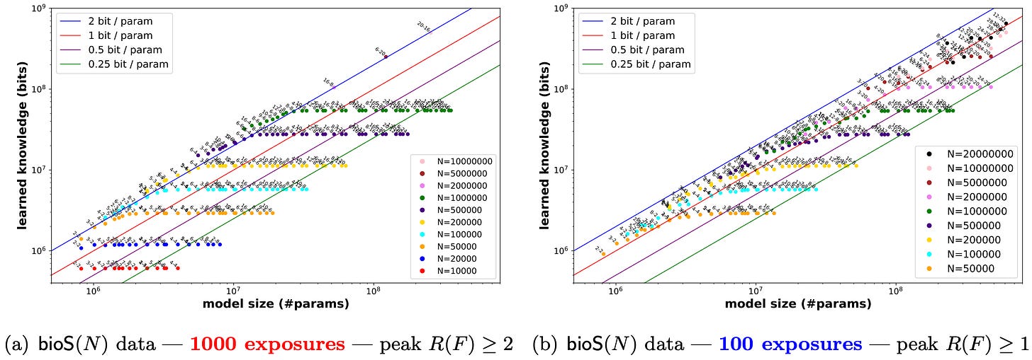
So what happens when you train a bunch of models of different sizes for different numbers of passes through these facts? It turns out that models consistently saturate at just over 2 bits of knowledge per parameter. Not all architectures achieve this bound, but none of them significantly exceed it. Each dot below is a (num layers, num heads) heads tuple for a GPT2-like model. For each number of facts, some architectures fall along the 2 bits/param line—just above it with 1k epochs and just under it with 100.
These same patterns hold for LLaMA/Mistral-like networks, not just GPT2. It also works with GPT2’s MLPs made 4x smaller or eliminated completely.
If you only show the models the facts 100 times instead of 1000, architecture changes start to matter though. Getting rid of the MLPs is especially bad.
In this low-training regime, you can close the gap between GPT2 (better) and LLaMA (worse) by making LLama use a standard MLP instead of a GLU, tying the input embeddings and output softmax, and using the GPT2 Tokenizer.
They also find that quantizing models to int8 doesn’t hurt the 2 bits per param result, while quantizing to 4 bits brings the peak down to ~.7bits/param. It’s not clear whether this is inevitable though or just a limitation of how the quantization happened.
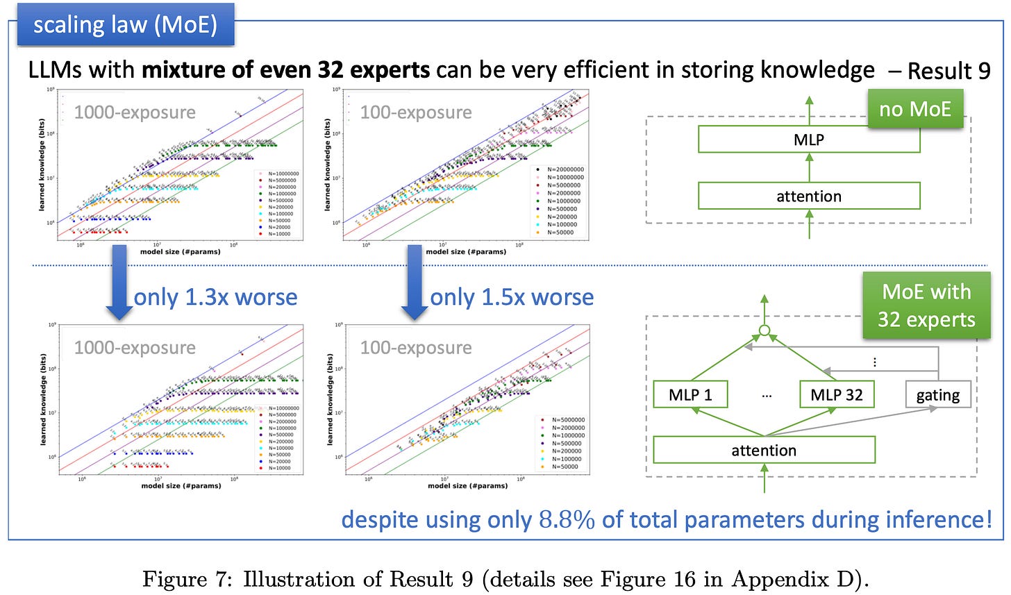
They also investigated what happens when you have 32 experts (topk=1, expansion_ratio=1) instead of a regular MLP (expansion_ratio=4). Despite being super sparse, the MoE only gets 1.3-1.5x fewer peak bits per param. The ratio also gets closer to 1 as the amount of training increases. This suggests to me that the experts might just be undertrained, see they’ve each seen about 1/32 as much data.
Finally, they explored what happens when you add in a bunch of “junk” data. Here, “junk” means the same sort of synthetic data, but drawn from a vast set of names such that you almost never get repeats—just a bunch of one-off facts.
First, making only 1/8 of your dataset non-junk can hurt the model by way more than a factor of 8. This ratio does improve as you keep training though, and eventually the model focuses on the non-junk (repeated) knowledge.
In contrast, if the junk data uses a much smaller set of names in its facts (so that it’s much more repetitive than the regular data), the capacity ratio isn’t affected much. This suggests that deduplicating your dataset might be much less important than removing one-off claims in the data.
If you can’t filter out the junk, you can at least help the model learn to ignore it by prepending sequences with a special token to indicate whether they’re from the regular distribution or the junk distribution. Given this cue, the model learns to ignore the junk.
I see a few actionable takeaways here:
It might help to prepend a “domain” token to your sequences telling the model what data source they’re from (e.g., wikipedia). Unclear what you do with this at inference time—might need to specify the “domain” as part of your prompt.
It might be more important to filter out non-repeated data than often-repeated data.
MoEs seem to need more training per param than dense models, though they’re surprisingly resilient to not having this.
We probably won’t get below 2 bits per parameter when compressing models without a large drop in model quality.
I also just feel like this is one of those papers I’ll keep coming back to as data to be explained when new science-of-deep-learning papers come along.
Lastly, I’m curious if we can push past 2 bits/param with more training. I could imagine that, say 10T tokens
Scaling Laws for Fine-Grained Mixture of Experts
Should you have bigger experts or more experts in your MoE model? Or more generally, how does your loss scale with expert size and count?
They consider in particular the effects of a “granularity” parameter, where G > 1 corresponds to chopping up each expert into G smaller experts with the same total parameter count.
They also consider the ratio of params in all the experts to params in a typical FFN with one expert and G=1, which they term the expansion rate. In typical MoEs, this is just the number of experts. But with more, smaller experts, we have to divide by the granularity G.
So what do they find? First:
There’s a power law relationship between granularity and loss (straight line on leftmost subplot).
Using a granularity of 4 doesn’t mess with the normal power law scaling wrt param count (straight lines in middle subplot).
Different granularity values don’t change the returns on training for more tokens (lines all similar in the right subplot).
Based on these interactions with the granularity G (or lack thereof), they find that a certain formula involving some power law relationships fits their observations:
This formula turns the granularity into a multiplier on the loss contribution from the parameter count, as opposed to contributing a separate loss term. Otherwise, it looks like the typical irreducible loss + additive param count loss + additive {token, step} count loss.
In practice though, you might not want the most granular routing possible because it starts to hurt your hardware utilization. This is because you’ll have:
More data transmitted into your all-to-alls to route tokens to and from experts
More activation memory for all your different copies of the tokens (at least with expert parallelism)
Smaller experts, which means smaller matmuls
More routing overhead
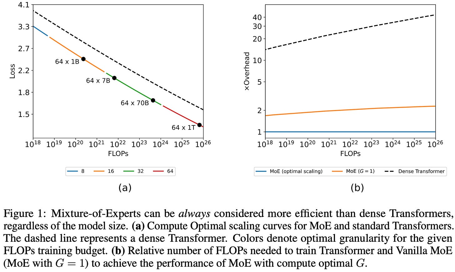
Taking into account the extra FLOPs from the routing, they derive optimal training settings for minimal loss subject to a FLOP constraint:
They also reconcile their results with those of Unified Scaling Laws for Routed Language Models by pointing out that you have to jack up the token to parameter ratio at larger model sizes. This previous paper held token count constant, which explains why they found diminishing benefits from MoE at larger scales.
We didn’t sweep enough hparams to get a formula, but we also found that more granular experts tended to do better—hence our use of 16 choose 4 in DBRX rather than 8 choose 2. The real limitation here though is not the FLOPs from routing, but the memory and allgather overhead; this means that I’d expect the granularities derived in the above table to be overestimates of what you should use in practice.
But either way, studies of how to scale are super important for maximizing and efficiency and model quality2, and this one is quite well-executed.
Mixture-of-Depths: Dynamically allocating compute in transformer-based language models
Why apply every transformer block to every token when presumably some tokens need more computation than others?
A classic approach to this is early exit, where we insert extra output heads at various depths and stop processing a token once one of the output heads has high enough confidence in its prediction.
But this approach adds a bunch of auxiliary heads (of size equal to our vocab size for language modeling…), yields stochastic work for each input, and induces weird and variable microbatch sizes across depths as tokens get dropped.
A cleaner approach is to only feed, say, 50% of the tokens into each residual branch. This yields a fixed, convenient batch size for each block and no extra output heads. And that’s exactly what this paper does.
The question is just how to pick the tokens to operate on. They solve this by performing a top-k operation with a learned router.
Or rather, they would implement it with a top-k op if they weren’t applying this to causal decoder models. In the causal case we encounter at test time, we can’t know if this time step’s token will be in the top-k until we see all the future tokens, which isn’t allowed.
So what they actually do is make the router a binary classifier whose labels are whether the token was in the top-k. This classifier makes an immediate operate vs skip decision for each token at each time step.
So how well does this work? At small scale, they can improve in wall clock time vs loss with mixture of depths. The best setting seems to be only applying their method to every other block, but skipping those blocks for 7/8ths of the tokens.
The way to get better results out of their method isn’t necessarily to just apply it to a given architecture though. You want to scale up the parameter count to compensate for the reduced FLOPs/token.
You might notice that all of the above results are use training loss where the ground truth top-k routing applies. What happens during autoregressive sampling, where we’re forced to switch to our trained binary classifier? Well…looks like we’re fine?
Finally, they test whether their Mixture of Depths (MoD) method plays nicely with Mixture of Experts (MoE), which they together refer to as MoDE. There aren’t super precise scaling formulas here, but it looks like the benefits from each compose. It’s not clear whether you’re better off combining them in the most obvious way or fusing the MoD and MoE routers; however, the latter is apparently better than just reducing the capacity factors and relying on token dropping to jankily approximate MoD.
We’ll have to see whether other people can reproduce it, but this seems like a significant win. And I’m bullish on this working since we’ve seen evidence for even more extreme token dropping in vision transformers.
Another benefit of this method that they didn’t really talk about is the big inference-time speedup you’d get during batch size 1 autoregressive decoding. Since you’re generating one token at a time, any block that the token skips requires zero work, including loading in the weights from RAM. With 12.5% of tokens selected in every other layer and no routing overhead this could get you a 1/(.5 + .125*.5) = 1.78x speedup.
Interestingly, this benefit disappears with speculative decoding or large-batch-size decoding, since you only get to skip loading the weights if all the tokens at this generation step skip it.
Side note: this was fewer papers but more depth than usual. How do you all feel about this?
I made this up but the rough idea came from a conversation with Trevor Gale, author of MegaBlocks (and other projects).
Not that these are different when you have a finite budget


I like the depth, but I also like the breadth of previous posts. You could do a few in-depth summaries and then just list some other good papers, maybe with a one-sentence reaction?