2022-10-16 arXiv roundup: Augmentation scaling, Better CNN initialization, Transformer sparsity
This newsletter made possible by MosaicML. Also thanks to @andrey_kurenkov (author of The Gradient) for recommending this newsletter on Twitter!
How Much Data Are Augmentations Worth? An Investigation into Scaling Laws, Invariance, and Implicit Regularization
A ton of cool experiments on the effects of data augmentations and when you should use different ones.
One observation is that different augmentations help in different data regimes. With not much data, aggressive augmentations are better. With more data, conservative augmentations like horizontal flipping are better. Seems like a bias-variance tradeoff wherein distorting the true distribution is worth it for small datasets to get more coverage, but not worth it for large datasets.
Augmentations have different effects across different architectures, but the relative effects of each augmentation are fairly consistent.
For OOD data, having a few augmented samples during training can be better than any number of in-domain samples (see the curves going to infinity on the right).
Interestingly, augmentations help OOD accuracy even if they don’t capture the correct invariance. E.g., horizontal flipping helps with rotated test data.
This might have to do with augmentations acting as a sort of regularization. E.g., augmented samples yield higher gradient variance late in training.
More aggressive augmentations also make the network settle in flatter minima—especially with small datasets.
Overall, this is one of the most thorough papers on data augmentation I’ve seen. I especially like the scaling curves in the first figure—suggests we could skip the hparam tuning and just pick our augmentations based on our dataset size, at least given some task-specific calibration.
The fact that augmentations sometimes beat infinite data also suggests that there’s more to the story than just acting as an expanded dataset. Maybe more evidence for Quality not Quantity.
Understanding the Covariance Structure of Convolutional Filters
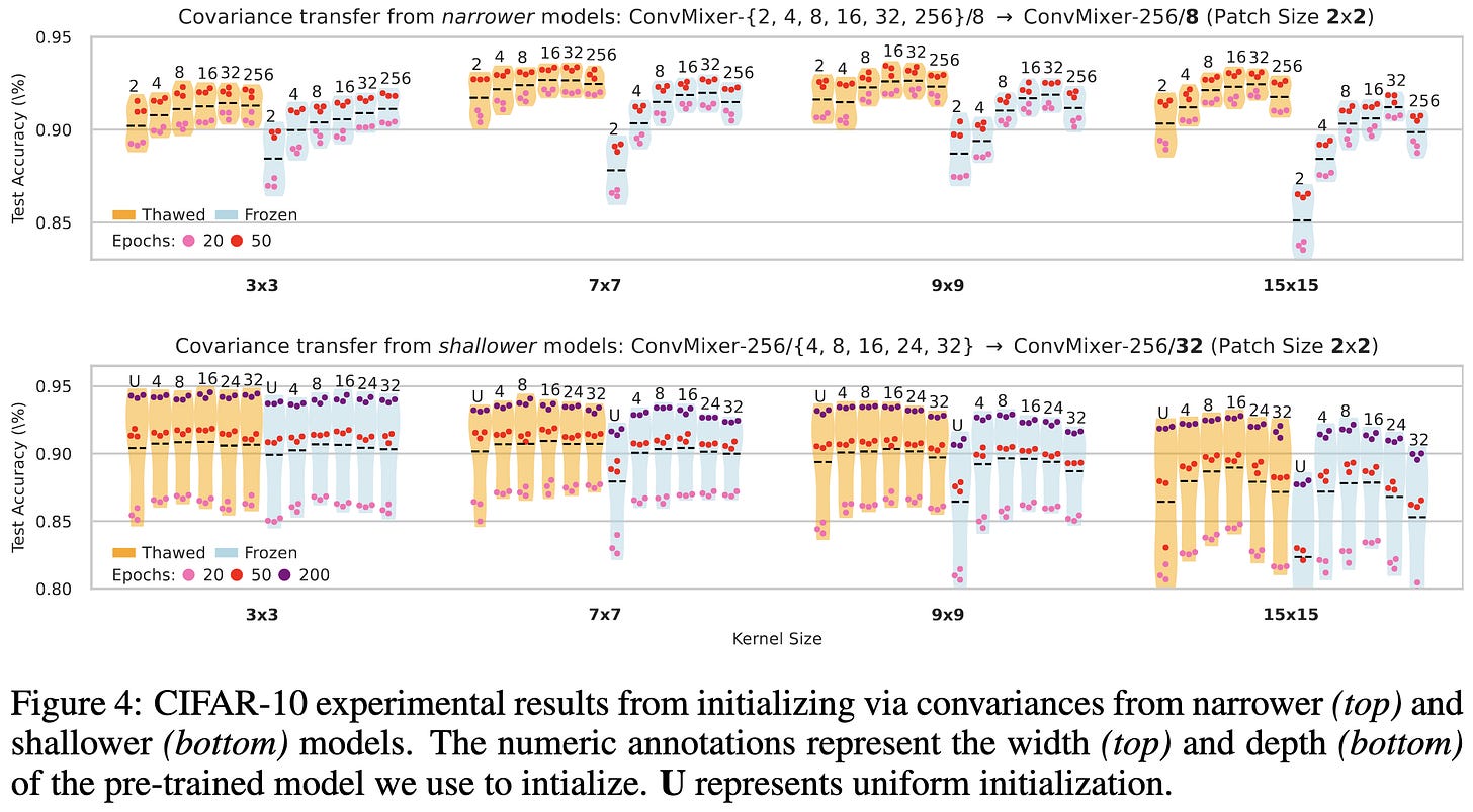
They observe that the depthwise conv filters in CNNs trained on CIFAR-10 tend to have particular statistical structure. By initializing models to have this structure at the outset, they get better accuracy with less training time.
More specifically, they find that you can treat the filters in each layer as vectors and model them as being drawn from a multivariate Gaussian. And you can mostly ignore the mean because it tends to be zero. So they sample from a Gaussian with a layer-specific covariance to initialize each depthwise conv’s filters.
Interestingly, this covariance transfer works even across models with different filters sizes or depths. For depth, they linearly interpolate source network covariances, with the interpolation based on the relative position within the source and target networks.
Taking it a step further, they propose directly generating suitable covariance matrices without using a source network.
With appropriate hyperparameters, this does even better than covariance transfer in some CIFAR-10 experiments.
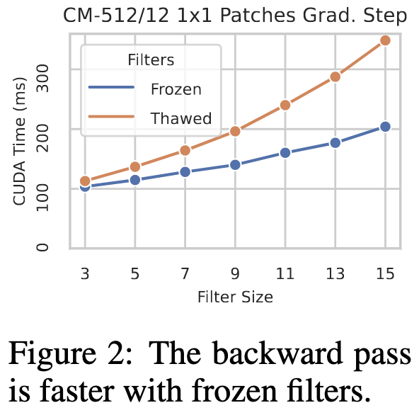
Pushing the limits even further, they consider freezing the filters entirely to speed up the backward pass.
On ImageNet, freezing is consistently worse than training, but surprisingly-not-terrible if you use their initialization. In general, their initialization beats the standard practice of uniform variance for all filter coefficients. Not clear if it beats transferring covariances from another network though.
This initialization doesn’t have the clean theory or nice properties of something like muParameterization, but might be an easy, practical win for CNNs with depthwise convs. Also makes me think that there could be a promising middle ground between using generic pretrained weights (which sometimes limit accuracy) and training from scratch.
Also makes me wonder if the effectiveness of simple pretraining tasks stems from getting weight / activation statistics right.
NoMorelization: Building Normalizer-Free Models from a Sample's Perspective
They propose to replace normalization layers with learned affine transforms + Gaussian noise.
This approach can work about as well as batch normalization on ImageNet. And it composes well with the gradient clipping and weight normalization proposed in the NFNet paper.
It does require you to tune the scale of the noise though. Networks that use batchnorm seem to tolerate more noise + a wider range of noise levels than layernorm networks.
I’d be surprised if this is better than batchnorm from an accuracy perspective, but eliminating the normalization overhead could be great for small networks.
Why self-attention is Natural for Sequence-to-Sequence Problems? A Perspective from Symmetries
There’s an elegant observation here. If you want your function to be equivariant to orthogonal transforms (i.e., rotating the input rotates the output), your function basically has to look like attention. More formally, all outputs have to be linear combinations of the input’s columns. This means you can equivalently write your function in terms of inner products between all the input columns, which is what attention does (with each column a token here).
Mass-Editing Memory in a Transformer
They consider the problem of directly editing factual knowledge in a decoder-only transformer like GPT-3. They improve on previous work by allowing far more facts to be edited without ruining the model.
More precisely, they consider (subject, relation, object) tuples and try to ensure that a given subject and relation are mapped to a certain object. This means ensuring that, at certain positions in the sequence, a particular class is the most probable at the output softmax. The goal is to modify the parameters as little as possible such that this happens.
Most previous approaches edit the parameters of a single layer. In this work, they distribute the edit across several MLPs that seem important for a given prediction. The importance is assessed using another paper’s heuristic.
Given the set of MLPs to modify, they perturb the weights to produce closer and closer approximations of the desired output. Since they use many MLPs, each perturbation can be small.
The exact math they use to change the weights is pretty involved, but it’s similar to a series of least squares problems, with each layer reducing some fraction of the gap between the current and target representation. What’s interesting is that it’s a fraction of the gap, not the whole thing—which ensures that each weight change is small.
By pretty much any metric you want to use, this approach outperforms previous ones once the number of desired edits gets large enough.
A related and more general finding is that certain categories of facts seem to be more amenable to editing than others.
This makes me hopeful that direct model editing could become a common supplement to (or maybe even replacement for) traditional training. E.g., I could imagine the ability to manually correct known failure cases being extremely helpful from an MLOps perspective.
S4ND: Modeling Images and Videos as Multidimensional Signals Using State Spaces
What happens if you lift S4 to operate on multi-dimensional signals by just applying it separately along each dimension?
Concretely, what if you swap out normal convolution or attention layers with outer products of 1d state-space models?
Well, it seems to improve accuracy at a given parameter count,
as well as video activity recognition—at least if you initialize the scale parameter appropriately.
It also seems to generalize well across resolutions, with an especially large improvement when training on low resolution and testing on higher resolution.
The downside is that it’s ~2x slower than the baselines. Although the authors point out that this gap could decrease with better implementations.
It’s not clear this is worth the speed and complexity cost, but state space models are super interesting and it’s great to see them extended to other classes of problems.
A New Family of Generalization Bounds Using Samplewise Evaluated CMI
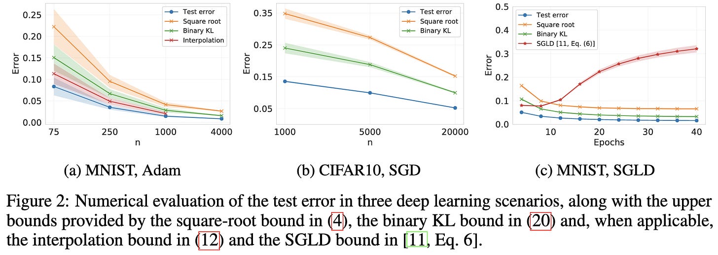
A new alternative to VC dimension, covering numbers, Rademacher complexity, uniform stability, etc., for constructing generalization guarantees. Their approach uses conditional mutual information, rather than properties of the hypothesis itself or the hypothesis class.
Impressively, the KL-divergence-based bounds they derive aren’t trivial on small-scale neural networks.
Seems like a handy tool for the theoretical toolbox.
Large Models are Parsimonious Learners: Activation Sparsity in Trained Transformers
As you might know, transformer activations tend to be really sparse. This paper examines this phenomenon in more details.
First, it’s not that most neurons are dead, but that nearly all neurons fire rarely. It’s only a handful that fire more than half the time.
Unsurprisingly, deeper and/or wider models have a higher number of nonzeros but a lower percentage of nonzeros. Also, I’m amazed at how consistent the nonzero counts are as you scale depth (left subplot)—this looks like someone just resampled the time series, with almost no noise.
Is this high sparsity just a quirk of transformers? Nope. Other model families, like ViTs, Mixers, and ResNets, also exhibit high levels of sparsity.
These architectures also exhibit the same pattern of wider models being sparser.
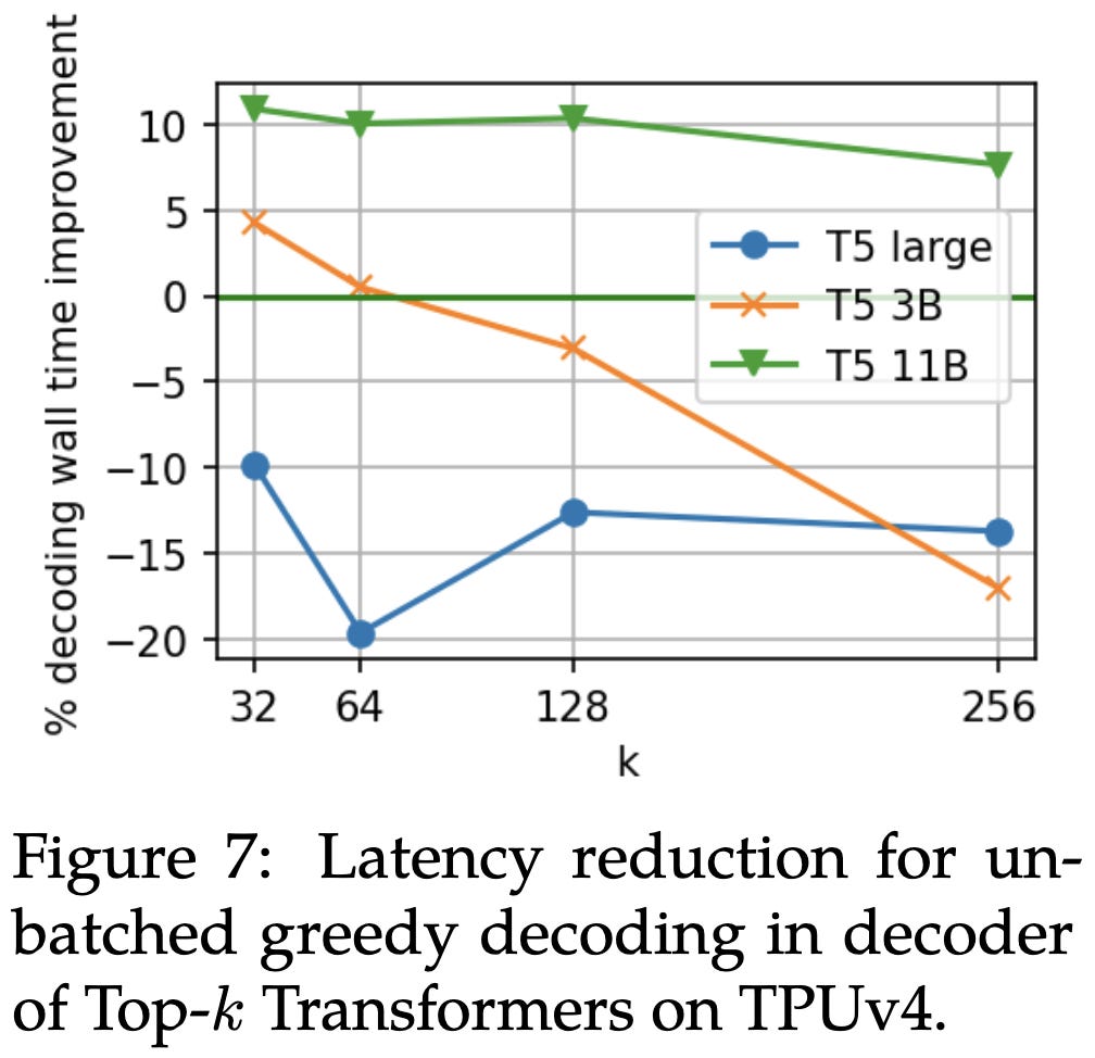
Can we exploit this high level of sparsity to speed up inference? Usually…not so much. But they propose a method of doing so. Their approach just entails applying a top-k operation to the hidden state within each of the MLP blocks. If you tune k, you can get nearly the same accuracy as the unconstrained model.
In return for this accuracy drop, you can get a small latency reduction on a TPUv4.
With the right k value, you can also get better OOD generalization than unconstrained models.
And a similar reduction in calibration error. Sadly, there isn’t a single value of k that works best for everything.
I’m not sold on top-k sparsity being broadly useful—I’ve tried it myself on small-ish models and it torpedoed the accuracy even for small k. But it’s great to see a paper with such thorough exploration of sparsity across so many models and experiments.
Learning to Optimize Quasi-Newton Methods
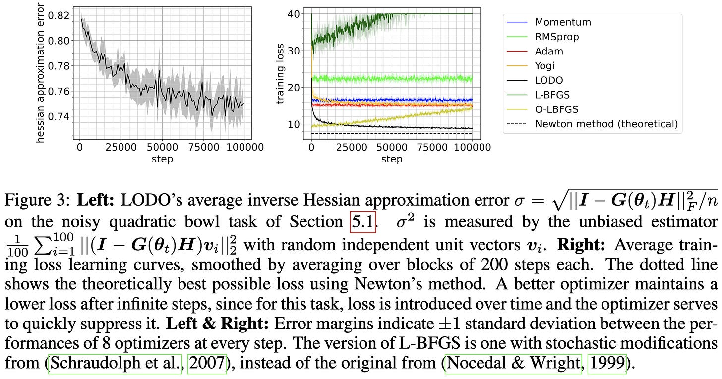
They use a structured, trainable approximation to the inverse Hessian for gradient preconditioning.
To train this matrix, they backprop all the way into the optimizer step. It ends up looking like preconditioned SGD updates to the model parameters and Adam updates for their approximate inverse Hessian. In the pseudocode, x is the model parameters and θ is the parameters for their matrix.
Their method provably learns the true Hessian for quadratic bowls under some assumptions, and does almost as well as Newton’s method in practice.
For generating MNIST images, it does about as well as other optimizers.
Not a ton of empirical validation, but I am optimistic about the basic idea of learning preconditioning matrices online in a lightweight manner.
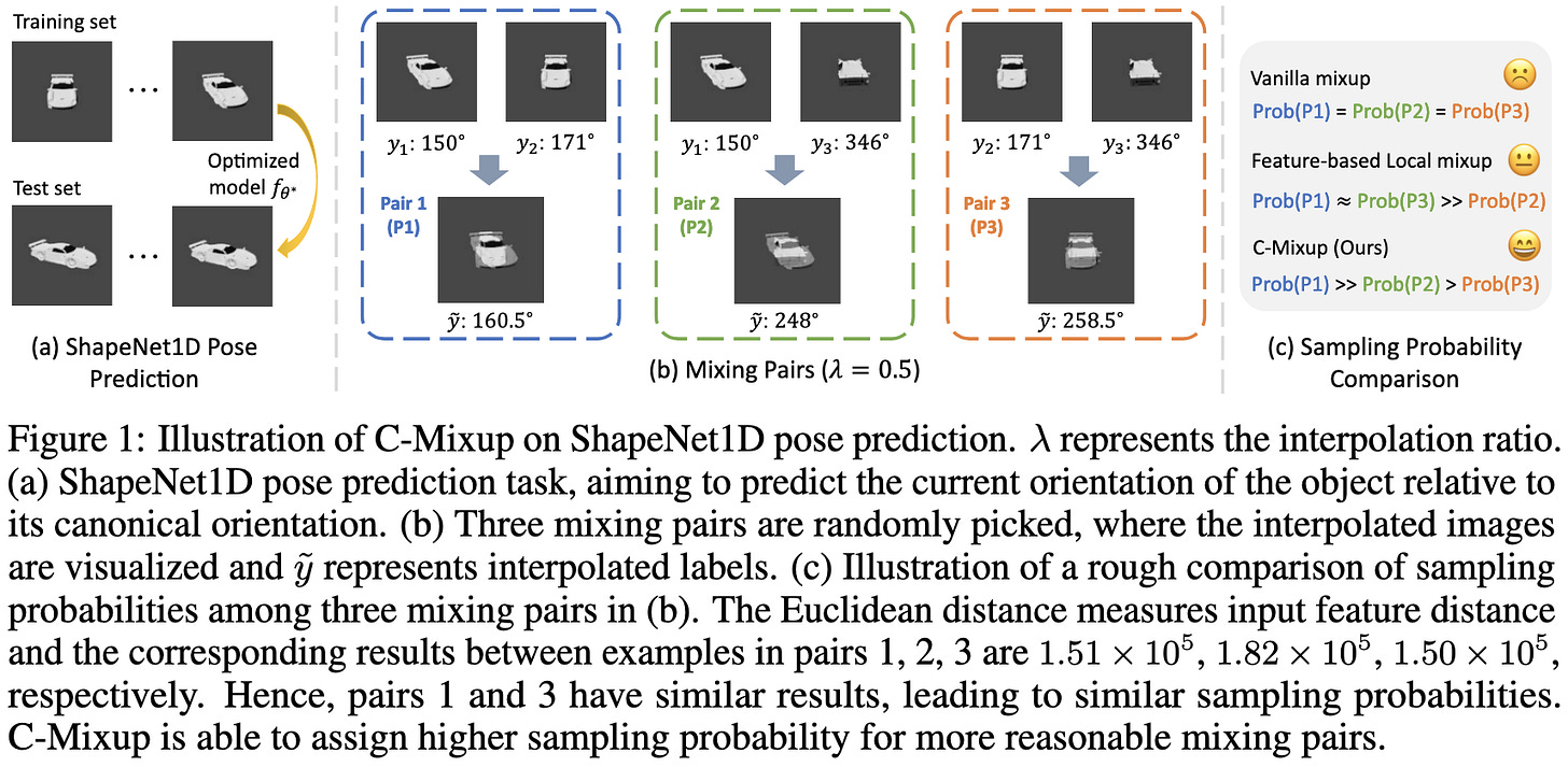
C-Mixup: Improving Generalization in Regression
When your targets are continuous, rather than categorical, regular mixup tends to produce unhelpful targets.
Instead, you should mostly just mix similar examples within a batch using a biased sampling scheme.
This helps accuracy across various regression tasks, both in-distribution and out-of-distribution.
Token-Label Alignment for Vision Transformers
When using CutMix with vision transformers, they change the label for each output patch based on which input patches contributed to it. They trace these contributions by examining the attention matrices.
This seemingly works better than other CutMix variants for DeiT-S on ImageNet.
Also yields a consistent improvement across many other vision transformers.
This method isn’t nearly as simple as regular CutMix and probably adds a fair amount of overhead, but might be worth it if the accuracy lift is as large as it looks.
Are Sample-Efficient NLP Models More Robust?
Nope.
A Generalist Framework for Panoptic Segmentation of Images and Videos
To get the segmentation mask for your image, make a Bit Diffusion model for masks that conditions on image features and an initial random noise mask.
Given a few helper functions, this is simple to implement:
It’s also fairly straightforward to extend to video; just condition on masks from previous frames.
Works almost as well as competing methods despite being way simpler.
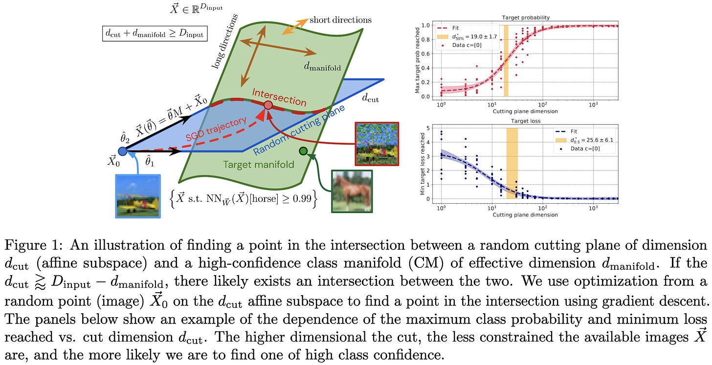
What does a deep neural network confidently perceive? The effective dimension of high certainty class manifolds and their low confidence boundaries
They propose a method to interrogate the dimensionality of the manifold representing each class in an image classifier. Basically, you use gradient descent to try constructing an input in a random, low-dimensional subspace that the model is confident is from a particular class. The lower the dimensionality for which this works, the higher the dimensionality of your class manifold.
This works because two random subspaces will tend to intersect iff their combined dimensionality equals or exceeds the dimensionality of the full space. E.g., if you can find a 32x32 = 1024 dimensional image that your model thinks is a “cat” in by only moving around in a 10-dimensional subspace, your “cat” manifold is probably at least 1024-10 = 1014-dimensional.
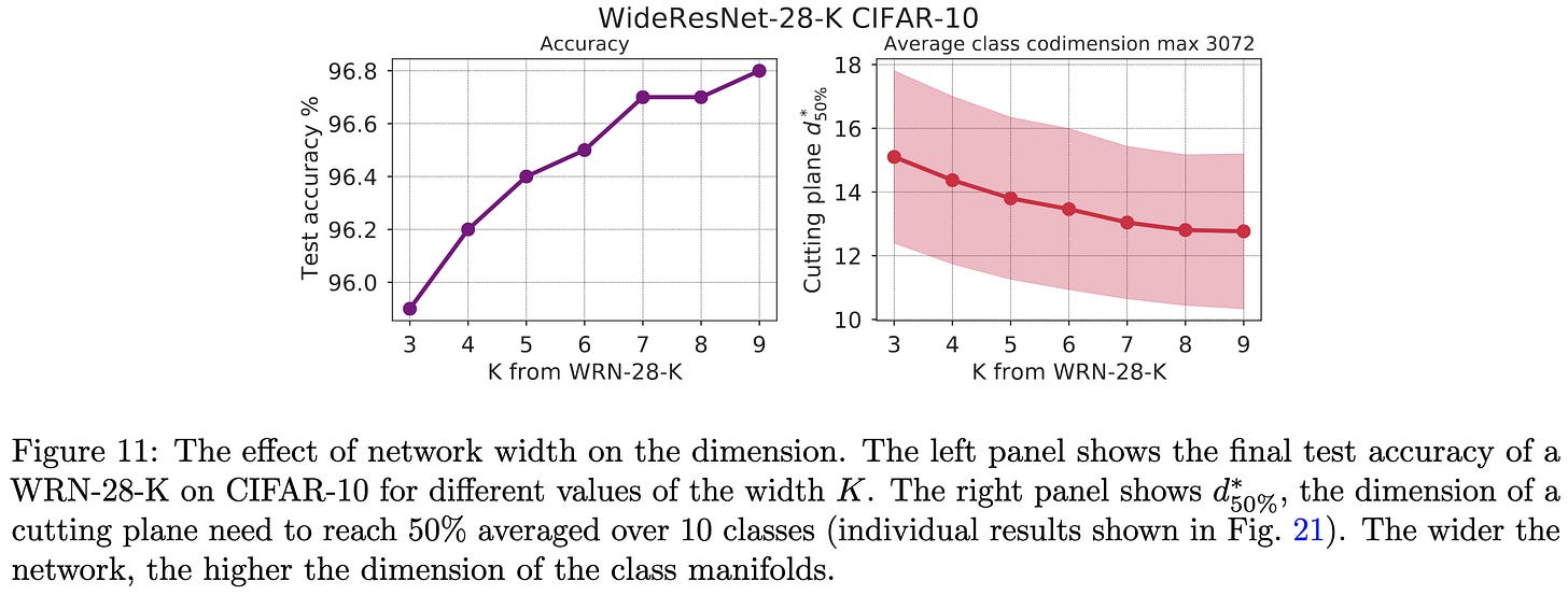
This Subspace Tomography method lets them show that class manifold dimension is correlated with all sorts of nice properties of the model, like accuracy and robustness.
Seems like a nice tool for probing neural nets.
SGD with large step sizes learns sparse features
If you’re using MSE loss, SGD is equivalent to gradient descent with random label noise. And the variance of this noise is both proportional to the loss and the inverse square of your dataset size.
They use this to argue that SGD might have some implicit bias towards sparse activations. They also argue that learning rate warmup helps with SGD’s implicit regularization.
Understanding the Failure of Batch Normalization for Transformers in NLP
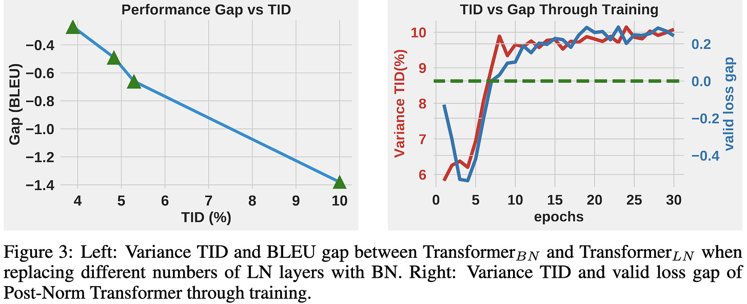
They find that batchnorm works just as well as layernorm for training, but does way worse at test time. Why is this?
Mostly deviations between the global mean and variance and the per-batch mean and variance. These deviations are small for some vision tasks like CIFAR-10, where batchnorm shines, but big for NLP transformers.
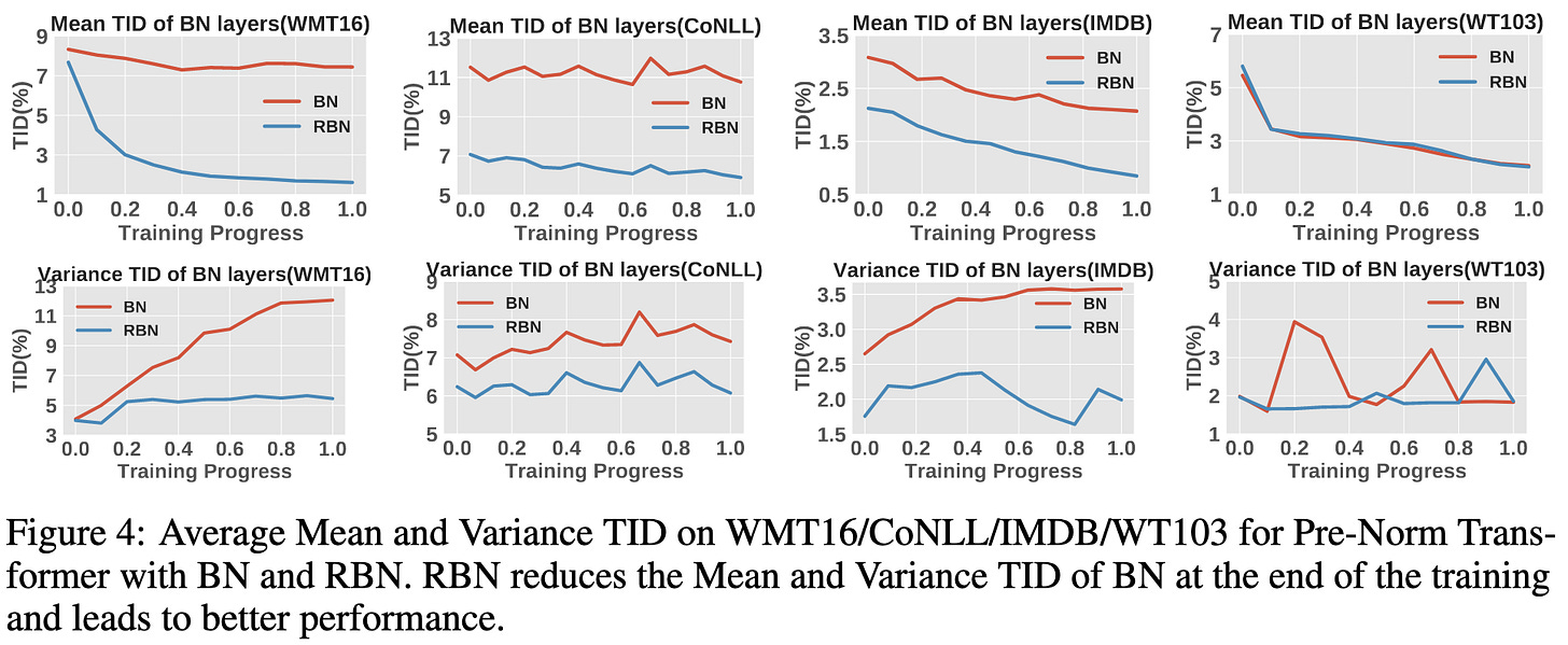
They propose a statistic called the Training Inference Discrepancy (TID) to quantify this global vs per-batch deviation and show that it correlates well with test-time metrics.
Based on these findings, they propose auxiliary losses to make the batch means and variances more closely match the global averages. They call this approach Regularized BatchNorm. It successfully reduces the TID statistic.
With good hparams for the extra loss terms, they can consistently beat layernorm and vanilla batchnorm for transformers with their RBN.
I can’t tell if the improvements are real or just a product of adding and tuning another hparam, but I really like their analysis of why batchnorm fails for transformers in NLP.
They didn’t frame it this way, but my takeaway from there being high variability in the variance is that the skewness, kurtosis, etc. are higher for NLP tasks/models than vision ones. Curious how much of this is a product of dataset statistics vs multiplicative interactions (attention) vs other factors.


