2024-8-4 arXiv roundup: LLama 3.1, training a 100T biological neural net
In case you’re wondering what I’ve been up to instead of posting for the past couple months, I was kicking off a training run for a 100T parameter biological neural network:
The dev team is healthy and the training run is hitting its quality targets. But boy are there a lot of failures to debug late at night…
The Llama 3 Herd of Models
In case you missed it, Meta released a family of models that are about as good as the best proprietary models.
This is a huge development for the field and also 73-page paper so…today’s post is mostly going to be about this paper, with less coverage of the literature in general.
Architecture
What’s interesting here is that it’s not interesting—just a vanilla transformer.
Of particular note is that they didn’t use sparse mixture of experts (MoE), which has a strong track record of improving cost-quality tradeoffs. This suggests they’re serious about the “becoming a standard” angle, since it’s much harder to do training, finetuning, and serving well with MoE.
It might also be a result of their interconnect bottlenecking their training on gradient communication, which would mean their training time is proportional to the parameter count. This would make MoE a bad deal during training.
Scaling
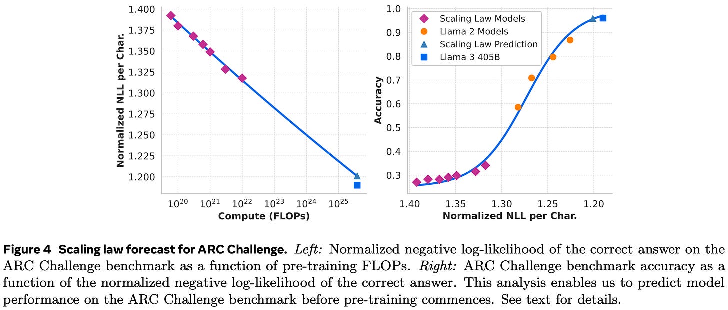
They’re trying to predict (and control!) benchmark numbers—not just pretraining loss—through their scaling choices.
To make these predictions, they often fit a sigmoid to downstream metrics like accuracy that saturate. Basically a generalized linear model.
They ran their own scaling experiments and didn’t just use the Chinchilla constants. The power law fit they get is pretty good, but there does seem to be a little curvature (meaning you want a higher token to parameter ratio at higher compute budgets).
They massively overtrained the small models but the 405B model is slightly undertrained based on their scaling results.
Infrastructure
They trained on 8 pods of 3072 H100s, with full all-to-all connectivity within each pod but 7x lower bandwidth across the pods. They only used 16k gpus at a time though (not 24k), possibly because this is a production cluster rather than a research cluster.
They only have two 8xH100 boxes per rack. This is pretty standard and probably a result of thermal limits. This low density is mostly okay because space is cheap compared to hardware, but having everything spread out can require you to buy more expensive cables to deal with signal attenuation.
They have their own fork of NCCL and their own ECMP variant.
They saw 1-2% speed variations based on time of day as a result of temperature changes. Just in case you thought your own profiling attempts didn’t have enough lurking variables.
Here’s their overall breakdown of outages/interruptions. They nominally trained for 885k H100-days and had 268 GPU hardware failures, for a GPU-level MTBF of about 3300 H100-days. This seems…way too long. Or maybe Meta is unusually good at datacenter design? Either way, it’s still a pretty high failure rate since you can’t hot swap the cards in an SXM box—you need 0 of 8 to fail for the server to work, so each server will fail a little less than once a year at this rate.
Despite the failures, they got >90% training uptime with only 3 instances of heavy manual intervention in 54 days. Getting your uptime this high is really hard to do.
They did a ton of work to reduce job startup and checkpointing times. E.g., they checkpoint to a giant SSD cluster with 2TB/s of sustained bandwidth.
Part of their ability to fix and prevent issues came from integration between their NCCL fork and PyTorch to get more detailed debugging information.
Sharding and Parallelism
They’re doing 4D parallelism with {tensor, context, pipeline, data} parallelism. These are in order of more local → more global. The TP (and maybe the CP?) are intra-box while the DP is inter-pod.
They didn’t need any activation checkpointing. But to achieve this, they did need to manually control some tensor lifetimes and mess with some NCCL details (like TORCH_NCCL_AVOID_RECORD_STREAMS).
They do interleaved pipeline parallelism, where each group of machines handles more than one pipeline stage. This reduces pipeline bubbles.
Their context parallelism just plain allgathers the keys and values right there on the critical path. But this is okay-ish because the KV tensor is small thanks to grouped query attention.
They use FSDP in Zero-2 mode, not Zero-3 mode. I.e., they keep the weight tensors materialized after the forward pass instead of re-gathering them in backward.
They use f32 gradient accumulation, including for their reduce-scatters.
Overall, they get around 40% MFU. You’d like 60%+ for a dense model within a single pod, but considering that they have to allreduce across pods and pay other scale taxes, this is impressive.
Pretraining
Over the first 252M tokens, they increased the batch size from 4M to 8M tokens and the sequence length from 4096 to 8192. They later increased the batch size to 16M tokens after 2.87T tokens.
They dynamically adjusted the data mix during training based on how intermediate evals were looking on downstream tasks. They also added fresh web data late in training to increase the knowledge cutoff.
They did 800B tokens of long context pretraining, gradually increasing the context length from 8k to 128k. They kept it at a given context length until short-context eval numbers fully recovered and the model solved “needle in a haystack” perfectly at the new length.
They used 40M tokens of extra high quality content at the very end.
Post-training
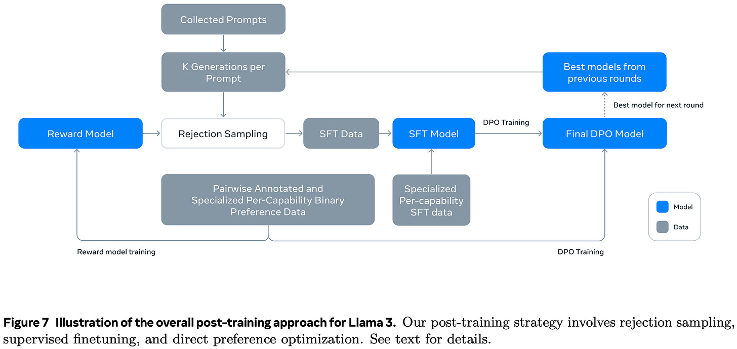
They did 6 rounds of iteratively post-training the model and using the new model to collect human feedback and generate possible responses. They use the best and worst1 responses (according to a reward model) as a contrastive pair for supervised finetuning.
They chose DPO over PPO since it’s not only more compute efficient, but also “performed better, especially on instruction following benchmarks like IFEval.”
They let human annotators edit responses in addition to rating them, and treat edited responses as a separate, higher tier of quality in their contrastive training.
Since most of their post-training data is LLM-generated, they add a bunch of rule-based cleaning steps to account for the LLMs’ quirks. E.g., they downsample outputs that start by apologizing.
Even for real data, they have elaborate pipelines that try to deduplicate documents, score them for quality, and estimate their difficulty. Within a given topic cluster, they greedily take documents that appear different from documents added-so-far in order of quality * difficulty.
Besides the synthetic data generation loop, they have a bunch of static, high quality data they’ve collected. Some of it is offline synthetic data that’s used to help with particular capabilities like coding or function calling.
Downstream task capabilities
Coding
They forked the model near the end of training and did continued pretraining on 1T tokens of code-heavy data to get a “code expert” model. They then post-trained this model much like the main model. This code expert lets them generate millions of synthetic code-debugging chats.
They generate their code data by:
Seeding a prompt with some real example code as inspiration to get diverse but realistic coding problems.
Having a model try to solve the problem and generate tests for it.
Filtering out responses that fail linting or the tests.
For code examples generated during the post-training rejection sampling part, you can’t always pull out the code cleanly. So here they just use an LLM as a judge. They also go out of their way to clean up the most challenging (and therefore valuable) examples so that they pass this filter.
They augment their set of coding examples by translating problems between different programming languages.
Multilingual ability
They mostly didn’t train on machine translations, but made an exception for math/reasoning data. This data didn’t hit as many quality issues when translated, maybe because there’s less cultural context or linguistic subtlety here.
They turned multilingual NLP datasets for various tasks into chats.
They used parallel texts from stuff like Wikipedia pages.
Math and Reasoning
They took a ton of mathematical documents and turned them into questions and answers for supervised finetuning.
They manually looked at what the model was bad at and got humans to generate training data to help with that.
They learn stepwise reward models to filter out data with incorrect reasoning traces and Monte Carlo Tree Search to generate attempted reasoning traces.
They prompt the model to generate code to embody its reasoning and filter out responses where the code is broken.
They try to get correct examples by prompting the model to fix broken ones.
Long Context
With long contexts, they mostly want the model to be good at question answering, summarization, and coding.
Almost all the data is synthetic since it’s so slow to have humans annotate it.
For summarization, they hierarchically summarize 8k chunks, then summarize the summaries, and so on.
For question answering, they have the model generate question-answer pairs based on random 8k snippets from long documents, but then use the whole document as part of the sample. They also generate some QA pairs based on their above generated summaries.
For long-context coding, they rip out a file from a repo and have model try to generate the file based on how it’s used in other files.
They use a 999:1 ratio of short-context to long-context data to trade off short- and long-context output quality.
Factuality / Hallucinations
They generate training data for “knowing what you don’t know” by generating factual questions from snippets of the pretraining data and using an LLM to check whether generated answers are correct or not.
Function Calling / Tool Use
The models are trained to call a search engine API, call the Wolfram Alpha API, or invoke a Python interpreter. They’re also trained for zero-shot tool use given just an in-context function signature and docstring.
All their tool use is executed through the Python interpreter. There are custom functions for each tool it can use, and new tools should be Python functions.
They *don’t* use model generations plus rejection sampling here—just human annotations and SFT on tool use examples from previous Llama 3 models.
Inference
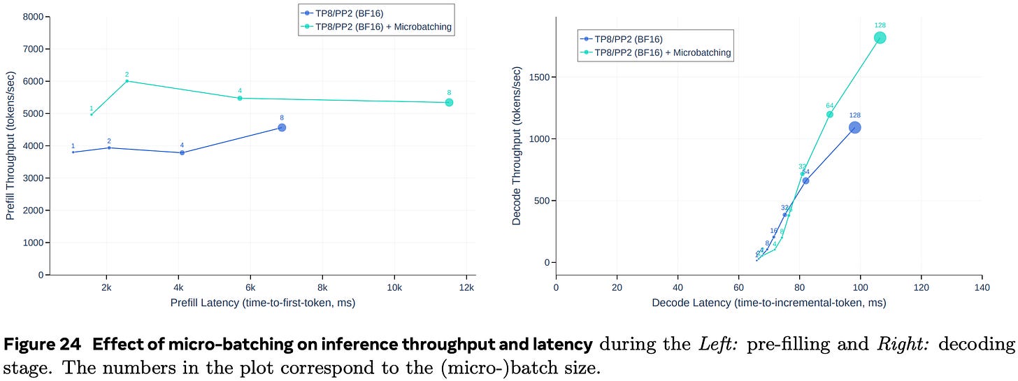
You can’t fit the 405B model on 8 H100s in bf16, so they use pipeline parallelism. This is probably the least bad option, but gets wrecked by batch size 1 inference. You not only pay for 2 nodes, but only get to use the hardware of 1 of them at a time.
With fp8, it fits on one node and you get a big cost + speed win.
The first surprising part of their fp8 quantization is that they clamp the row-wise scale factors at 1200. This avoids an edge case where high-entropy tokens cause large activations, which in turn cause underflow in their row if the scaling factor isn’t clamped.
The second surprise is that they don’t quantize the attention parameters.
I didn’t even get to the vision or speech sections here, but you’ve been reading this for a while and I’ve been reading this paper for hours so I’m gonna truncate the methodology summarization here.
Analysis
What stands out to me more than anything is the huge amount of synthetic data involved. Synthetic data is at the core of everything after pretraining. It’s also a result of highly customized pipelines. We used to incorporate domain knowledge by engineering features, but now we’re instead engineering sampling and filtering pipelines.
I’d expect these synthetic data pipelines to get better as models improve, which has three interesting consequences:
There is now a clear, tight feedback loop of AI progress directly causing AI progress in a virtuous cycle. And there’s no end in sight.
It’s likely that there will be way more inference compute than training compute in the future, since only a small fraction of the generated data passes the filters.
We could be in for winner-take-all dynamics, where the organizations with the best model can generate the best data.
Although Llama 3 405B being open-weights means that no one actually has this structural advantage at the moment. The advantage instead lies in the proprietary code and internal know-how that lets you actually run the data generation pipeline.
There may be a more efficient way to turn money into model quality. Even with Chinchilla-optimal scaling, you get brutal diminishing returns where you have to do ~64x as much compute each time you want to halve the reducible error.2 So what you actually do is allocate some of your money to raw scale, and some to extremely expensive labor to shift the cost-quality curve. But it could be the case that the marginal returns on compute for synthetic data are higher than either of these other investments, at least to a point.
In terms of non-technical implications…having one player just give away for free what other firms are spending building of dollars to produce tends to go poorly for the other firms. I know people at most of the foundation model companies and I hope things work out well for them, but the structural economics aren’t looking great—at least as long as Meta sticks to its open source guns.
The good news for foundation model companies is that:
Query volume is a structural advantage. More people are hitting [Azure] OpenAI than other providers, and this gives them both higher batching efficiency and more data.
If differentiation is impossible, brand becomes a moat. E.g., you can’t beat Coca Cola because there is no way to improve soda enough to overcome their brand power. Maybe the AI APIs will all be about the same and people will just use OpenAI or Google because that’s what they know about.
Meta doesn’t have that compelling a case for open weights compared to past examples, so maybe they’ll stop at some point. E.g., Google could give away Gmail, Google Docs, etc, because they had a clear path from user data to profit. But Meta doesn’t directly make more money from people using Llama 3. They just want to make their stack a standard and commoditize their complements (i.e., crush the firms who bid up the prices of GPUs and labor).
The sheer amount of revenue going into foundation model companies could get so high that even Meta can’t justify keeping up. We’re nowhere near this, but suppose someone builds a $100B dollar cluster. Could Meta really get enough marginal ad revenue from matching that to make it worthwhile? The digital advertising TAM is not as large as the “all knowledge work” TAM and this could start to matter.
The Illusion of State in State-Space Models
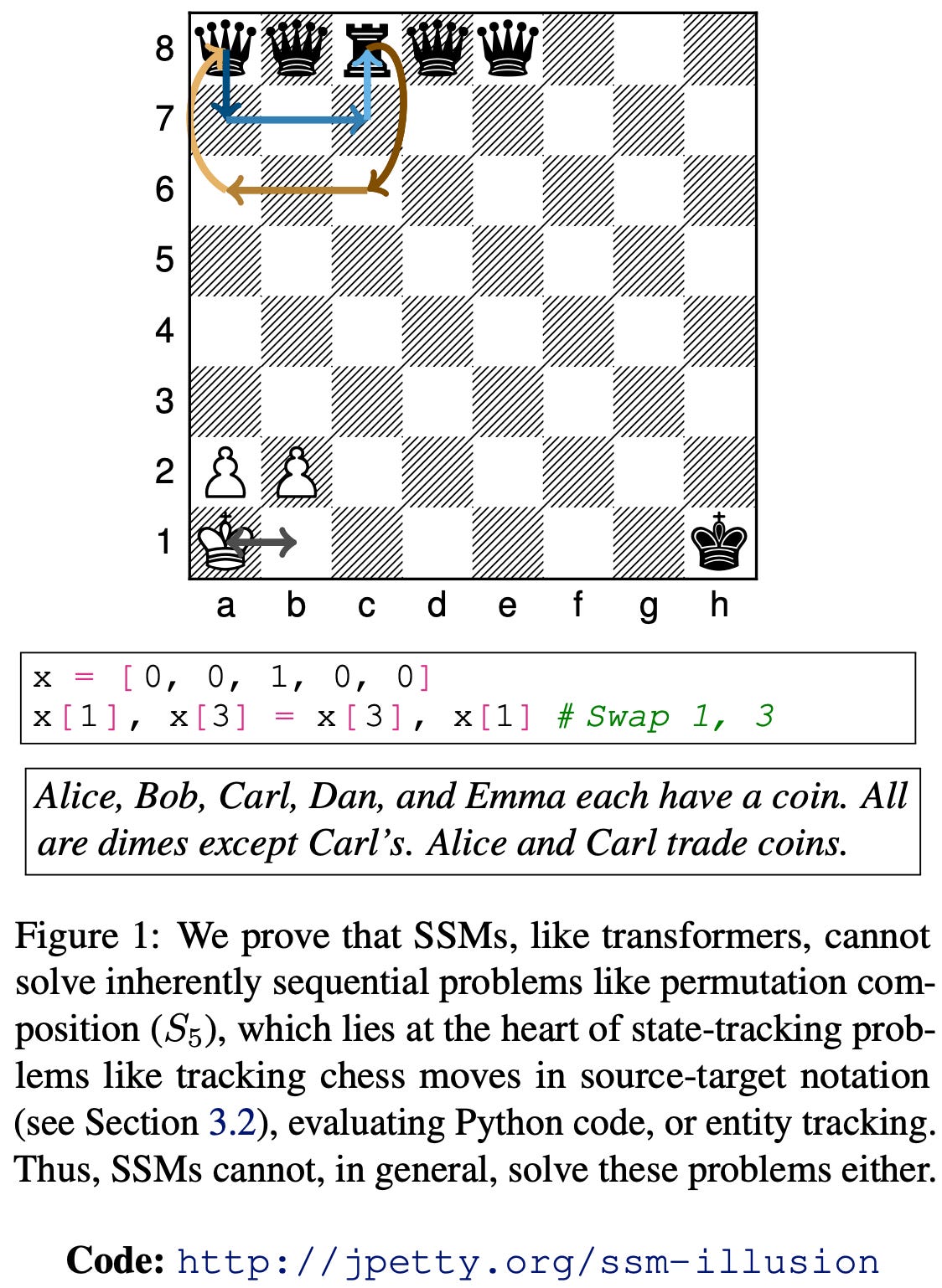
From a theory perspective, most state-space models can’t solve simple problems that involve tracking basic state. Examples include evaluating a boolean formula, composing permutations, or representing the current state of a chess board after a history of moves.
This also applies to transformers, but, interestingly, not RNNs.
This kinda makes sense given that SSMs can be expressed as convolutions. If your function can be expressed as a pure function of the previous layer with no sequential dependencies, it stands to reason that you can’t capture certain sequential dependencies.
Better & Faster Large Language Models via Multi-token Prediction
They add more heads to the LLM to predict future tokens kind of like Medusa, but they don’t necessarily use these extra heads during inference.
Instead, they just use this as a different training objective and find that it lifts model quality for large enough models.
They do show, though, that you can use the extra heads during inference as candidate tokens for speculative decoding. This can yield a pretty significant speedup in the best case.
It’s a bit unclear why this multi-headed training helps quality, but they conjecture that it has to do with emphasizing important tokens in the loss.
A little intellectually unsatisfying, but I’m always a fan of practical time-to-accuracy wins.
DiPaCo: Distributed Path Composition
This paper is a bunch of DeepMind people asking “what would it look like to build the most scalable training setup possible?”
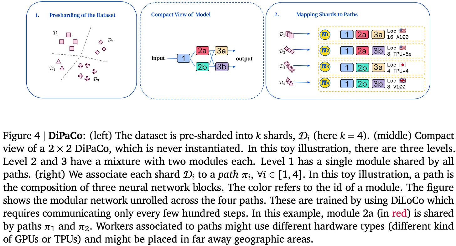
Their answer is roughly that each of your layers would be a mixture-of-experts, but with all the routing decisions determined at the input. You can think of a full sequence of routing decisions as a “path” through the model.
They also choose to route chunks of tokens and not individual tokens, optionally with different train- and test-time behavior. E.g., we might do more granular routing at test time or do top-k with k>1 during training to give experts more data.
The other big difference from typical MoE is that they materialize each possible path through the experts separately—maybe even on separate hardware in separate datacenters.
This is nice and parallel, but means that there are different copies of a given expert in different places. How do we synchronize them?
Their answer is using DiLoCo. This algorithm has each path optimize its params separately and then uses SGDM to sync across all the replicas, with the summed local parameter changes since the last sync treated as a gradient. This lets them sync weights rarely—maybe once every few hundred local steps.
To build this system, they largely lean on a smart task scheduler and Google’s distributed filesystem. This design is surprising to me because
usually we all live in SPMD-land with deterministic, synchronous semantics, and
usually we try to keep the filesystem or object storage out of the critical path.
For point (1), I’m not sure whether they’re getting sacrificing synchronous semantics and/or determinism. But for point (2), it looks like they’re syncing experts across paths so rarely that they can get away with using GFS and CPU parameter servers to read, combine, and broadcast all the local updates.
It’s a little unclear how to evaluate this approach since it’s so different from common practices. But it passes a bunch of sanity checks—e.g., you’re better off having bigger models and more data.
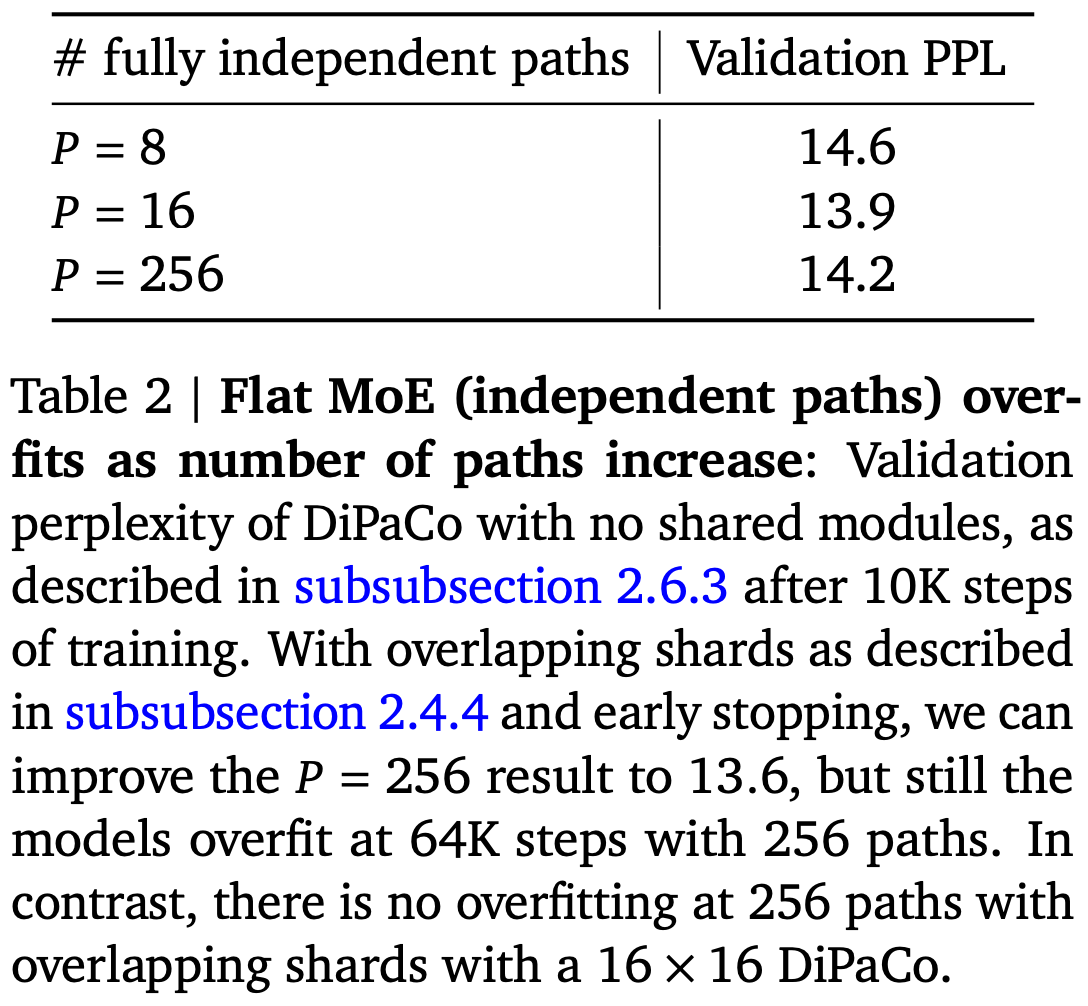
Similarly, they find that it does, in fact, help to tie parameters across the different paths, instead of just having each path be a separate network.
Side note: I like the below table because it backs up something I think I found but never looked at rigorously: if you scale up the expert count too high, eventually the reduced data per expert hurts more than the higher parameter count helps.
What I like about this paper is that it’s ambitious. There’s so much incentive to work on tweaks to existing practices, and it’s so rare to have people think from first principles about what the best case scenario is. And it’s rarer still for people to turn that thought into a real, working system.
Or maybe random other responses? I’m not sure.
With additive terms for data and parameter count scaling that take the form 1/n^.34, using 8x more data and 8x more parameters multiplies your reducible loss by 1/(8^.34) ≈ 1/2. This is the most efficient allocation, but still needs 8 * 8 = 64x as much compute.










Congrats on the new addition to the family, and also a more dynamic training round! Insights on llama3.1 are very helpful as usual, I am mostly impressed by the simple architecture to max training stability and the heavy use of synthetic data in post training.
Just started training my second 100T model and haven't had time to read the Llama 3.1 paper. Thanks for putting in the work 🙂