2023-11-26 arXiv roundup: Big potential wins, 1 bit per parameter, Simplifying transformers
Stella Nera: Achieving 161 TOp/s/W with Multiplier-free DNN Acceleration based on Approximate Matrix Multiplication
They built a crazy fast hardware accelerator based on my approximate matrix multiplication paper. By “crazy fast,” I mean they get 15x higher area efficiency and 25x better power efficiency vs conventional matrix multiply acclerators (think GPUs) when holding transistor technology constant. At ~1.5x better power efficiency per hardware generation, this is about 8 generations of gains at once.
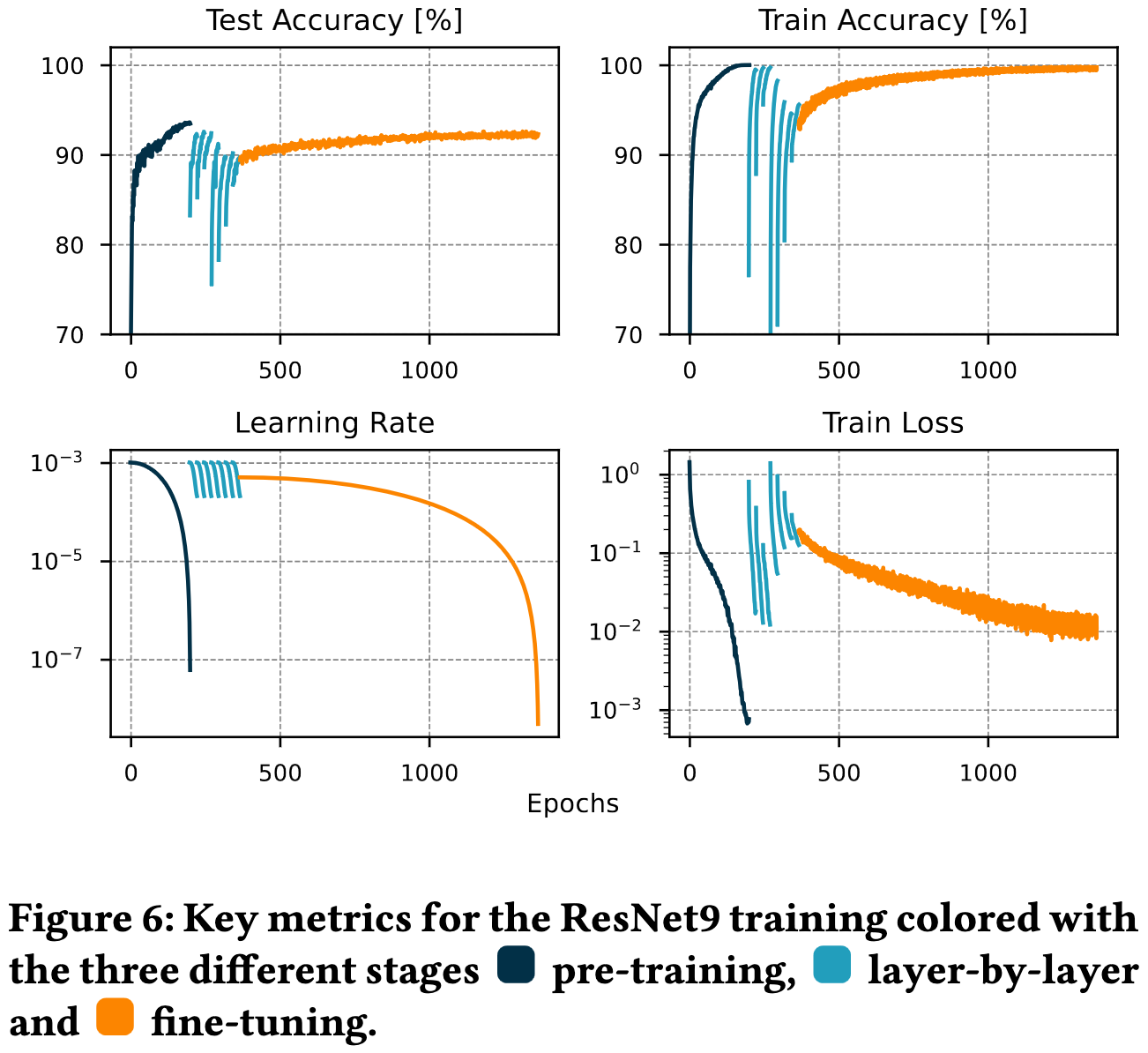
The catch is that they lost some model accuracy, at least for the ResNet-9 they tested on. And this is with layer-by-layer approximation of a pretrained model and subsequent finetuning, not just with post-training quantization.
That said, it’s probably a large net win; a rule of thumb I like is that you can trade 1% accuracy for 2x speed, so ~20x for 2% is much stronger than typical tradeoffs—though we of course need many more experiments and baselines to be sure.
So how do they achieve these gains?
Interlude: MADDNESS background
Before talking about their accelerator, we need to go over the approximate matrix product algorithm they’re accelerating. Basically, we’re going to approximate the product AB by lossy compressing A and B in a special format that’s smaller and that we can operate on super fast.
Common lossy compression techniques for this problem are pruning, quantization, and factorization. These help, but it turns out you can do way better with a different approach (spoiler: vector quantization).
The intuition for this approach is as follows: what if we knew that A only had a few unique rows that repeated many times?
In this case, we could just replace A with the set of unique rows and a bunch of indices, identifying which of the unique rows was in each position.
Given this representation of A, we could also compress B a ton. The observations here are:
a matrix product is just a bunch of dot products between rows of A and columns of B, and
the rows of A are repeated a bunch of times. So why recompute the same dot product when we could just memorize it?
So what we do is replace each column of B with a lookup table. Each entry in the table is its dot product with one of the unique rows. This is lossless compression for a given set of unique rows.
So now we’ve turned A into a bunch of indices and B into a bunch of tables. How do we multiply them? Easy—it’s just a bunch of table lookups. All we do is:
for i in range(A.shape[0]):
    for j in range(B.shape[1]):
        out[i, j] = B[A[i], j]
That’s it.
Now there’s one big problem with this: the matrix A probably doesn’t have a bunch of exact-duplicate rows. We’re going to solve this in two ways:
We’ll cluster the rows of A. This gets us prototypes/centroids instead of “unique rows.” The fact that a true row isn’t identical to its centroid is what makes the algorithm lossy.
We’ll split A into a bunch of disjoint subspaces and cluster within each subspace. Clustering won’t capture much of the variance in a 1024-dimensional space, but it can capture lot of it in, say, a 4-dimensional space. We’ll have many low-dimensional clusters instead of a few high-dimensional ones.
When the clustering algorithm is K-means, this algorithm is called Product Quantization (PQ).
This works super well and is a foundational algorithm in information retrieval.
The code to create the centroids looks like this, and runs in an offline training phase before we receive our matrices:
def learn_centroids(
    A_train, # training matrix; e.g., activations for training inputs
    num_subspaces: int,
    num_centroids: int = 16) -> array:

    N, D = A_train.shape
    subspace_len = D // num_subspaces
    centroids = empty(num_subspaces, K, D / num_subspaces)
    for s in num_subspaces:
        A_subs = A[:, (s * subspace_len):(s+1)*subspace_len]
        centroids[s] = k_means(A_subs, num_centroids)
    return centroids
At runtime, here’s how it encodes A:
def encode_A(A, centroids) -> array:
    N, D = A.shape
    num_subspaces, num_centroids, subspace_len = centroids.shape
    out = empty(N, num_subspaces)
    for s in num_subspaces:
        A_subs = A[:, (s * subspace_len):(s+1)*subspace_len]
        l2_dists = A_subs @ centroids[s].T - l2_norm(centroids[s].T, dim=0)
        out[:, s] = argmin(l2_dists, dim=1)  # N x 1
    return out
And how it encodes B1:
def encode_B(B, centroids) -> array:
    D, M = B.shape
    num_subspaces, num_centroids, subspace_len = centroids.shape
    out = empty(num_subspaces, num_centroids, M)
    for s in num_subspaces:
        B_subs = B[(s * subspace_len):(s+1)*subspace_len] # subs_len x M
        out[s] = centroids[s] @ B_subs  # 1 x M
    return out
to estimate dot products, product quantization just generalizes our single
out[i, j] = B[A[i], j]to a sum over the different subspaces:
out[i, j] = sum([ [B[s, A[i], j] for s in range(num_subspaces)])And that’s product quantization.
MADDNESS, the algorithm we’re accelerating, adds three optimizations on top of this:
It averages across subspaces at the instruction level instead of summing for better numerics.
It lets the centroids span across subspaces and jointly optimizes them using ridge regression, which makes the compression less lossy.
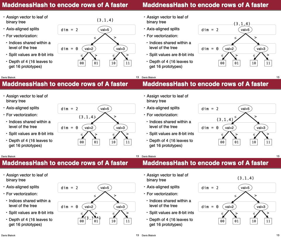
It uses probably2 the fastest locality sensentive hash function there is to assign rows to clusters, instead of the brute-force comparison to all centroids.
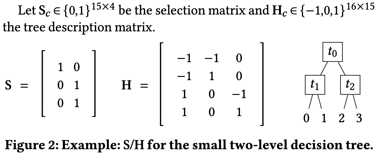
The third one is the most interesting. I won’t go over it but it’s essentially just learning a binary decision tree, assigning rows to leaves, and calling each leaf a cluster.
These changes let it approximate matrix products ridiculously fast even on current CPUs.
And this is without good hardware support. With better hardware support, it would of course be even better.
But is this algorithm conducive to hardware acceleration? Yes, very much so. This is because it:
Lets us do table lookups instead of multiply-adds. Multipliers scale quadratically in the number of bits involved and are pretty complicated circuits. Table lookups are just multiplexers, which are way simpler.
Compresses the matrices a ton, reducing memory usage.
Preserves the layout and access patterns of a dense matmul, including the tiling/data reuse. A MADDNESS kernel looks exactly like a dense GEMM kernel except that the matrices have different element sizes.
And now you understand the state of the art in approximate matrix multiplication!3
Hardware
So…back to the paper at hand. They add hardware acceleration to the centroid assignment function by loading the relevant indices in parallel and store-forwarding the left- vs right-child decision at each level of the tree. This gets them a throughput of one centroid assignment per cycle with a latency of four cycles.
They similarly accelerate the table lookups by using a multiplexer and a low-bitwidth adder. They tried fp16 table entries with fp32 accumulators, but found that int8 + int24 worked just as well.
They also introduce some algorithmic ideas to make the accuracy not terrible, since just naively approximating each layer in isolation goes badly. They:
gradually replace layers from beginning to end,
keep the first and last layers in fp16, and
relax the hash function assignment to be differentiable during finetuning.
I’m not too calibrated on energy dissipation numbers, but here’s how much they use for all you hardware people:
So what does this all mean?
First, the potential power and area savings are real. An H100 uses 400W to do ~2e15 int8 multiply-adds per second, for a total of 5 TOp/s/W. Meanwhile, this paper got 43 TOp/s/W. That’s over 8x better despite the former using 4nm process technology (~2021) while the latter uses 14nm (~2014).
But no one has managed to do this without accuracy loss, and probably no one will4. The reason is that vector quantization / table-lookup-based approaches almost always operate in the high compression regime. You need small tables to fit in registers or L1 cache, which means each table is, in practice, either 16 or 256 elements. This in turn makes the table indices either 4 or 8 bits. If we compress one scalar into 4 bits, that’s already aggressive scalar quantization. But if we’re compressing multiple scalars into 4 bits—that’s a lot of compression.
Putting it all together, the way I think about this is that:
Vector quantization nearly guarantees better space efficiency than scalar quantization. This is because vector quantization can learn to just scalar quantize as a special case, but exploits mutual information across dimensions if it’s there.
Consequently, MADDNESS and friends are strictly better than binarization, in that they’re more expressive but no more expensive.5
However, you can only compress a lot with vector quantization, not a little. So you probably need to train with more parameters/tokens to hold accuracy constant.
Vector quantization currently lacks support in tensor cores and other hardware, so it’s only useful today on CPUs and for bandwidth-bound operations like matrix-vector products.
I have like 95% confidence that vector quantization will win in the end, since the information per bit is so much higher. But it will probably take more papers like this before it gets on the roadmaps of major accelerator vendors.
Exponentially Faster Language Modelling
Here’s another ambitious paper that incorporates some similar ideas. It’s largely a follow-up to their recent Fast Feedforward Networks paper that applies this technique to a Crammed BERT and improves some details.
The basic idea here is to do extremely granular mixture of experts, with small slices of weight matrix columns (or even single columns) treated as experts.
To make this work, they:
Arrange the experts into a balanced binary tree, with each expert corresponding to a leaf node.
Have multiple disjoint trees + sets of experts, and sum the outputs from each.
Do soft routing during training. This routes every token to every expert, but with a small routing weight for nearly all experts.
Randomly flip the routing weights during training. E.g., if a token would give 90% weight to one child node and 10% to the other, this is swapped.
Add a “hardening” loss to anneal towards hard expert assignment by the end of training.
Here’s the training and test-time pseudocode:
When finetuning a pretrained BERT on GLUE tasks for 24 GPU-hours, they get almost the same accuracy as the dense model, even when only 12 out of the 4095 output features get activated for each token.
Because feature-level sparsity gets you both smaller inputs and smaller outputs, this can yield enormous speedups. You can’t really use the tensor cores once the experts get small enough, but with only 12 neurons used per layer, you can overcome this constant factor with sheer sparsity.
We’ll need to see clean {training time, inference time} vs accuracy curves and independent reproduction before we can be sure this is a real win, so here’s a spectrum of ways I think this could play out.
In the most optimistic case, there’s so much activation sparsity in common networks that this granular approach to conditional computation is usually just a good idea (at least for inference). It’s effectively the MoE-as-block-sparsity framing, with higher sparsity prioritized over higher utilization.
A moderately optimistic take is that they’ve found some combination of:
A better way of doing MoE routing, especially at large expert counts
More evidence that increased granularity in MoE experts is helpful.
More evidence that summing outputs from disjoint sets of experts is helpful.
And the pessimistic take is of course that, like the vast majority of papers, this won’t reproduce and/or won’t even look good once you understand the experimental details.6 The biggest question mark I see is that apparently their dense GPU baseline is their own extremely slow kernel. This is totally legitimate as a way to make the baseline implementation closely match their method’s implementation, but it does mean that the baseline is probably 10x+ slower than what you’d get normally.
In any but the pessimistic case, this has an interesting relationship to the vector quantization stuff above. Their differentiable binary trees could be exactly what we need to get tree-based hashing differentiable. Further, their finding that hashing input rows using multiple learned binary trees exactly lines up with what worked well in MADDNESS. Maybe just wishful thinking, but two groups arriving at similar solutions independently seems like mild evidence that there’s something there.
QMoE: Practical Sub-1-Bit Compression of Trillion-Parameter Models
Okay, I want more papers like this.
What I like is that they exploit the fact that we often have an explicit decompression step between loading weights from RAM and using them in our ops. When this is the case, you don’t need your compressed representation to just be quantized, sparse, or factorized—it can be the result of an arbitrary lossy compression algorithm. As I’ve said before, this buys you way more degrees of freedom and enables much better compression.
The overall setup here is that they do GPTQ on batches of experts, with ternary quantization in the most aggressive case. They then run this ternary encoding through the rest of their compression pipeline.
This pipeline uses dictionary coding with fixed codewords. The codewords are formed by computing the empirical probability of a zero in the ternary encoding and materializing the 2^16 most probable sequences of codes assuming the elements are iid and the +1 and -1 ternary values are equiprobable.
This lets them encode many weights with a single 16-bit code. One subtlety here though is that they also need to handle sequences of values that aren’t among the most probable 2^16. They do this by having variable-length dictionary entries, with each entry containing a header that stores how many symbols it contains. As long as all codes of length at most k are present in the dictionary for some k, this lets you encode any sequence of ternary values.
On top of this encoding, they sort these 2^16 codewords by estimated probability to maximize the number of cache hits they get. They also wrote a fused decode + matvec kernel to avoid an unnecessary roundtrip to RAM.
To make all this work, they had to solve some other hard problems along the way. E.g., they have to fetch the relevant weights lazily from disk to avoid CPU OOMs for trillion-parameter models.
Another enhancement they introduce is ignoring special tokens like padding when estimating the Hessians for quantization. They also ignore the tokens immediately preceding the special tokens.
Combining all these ideas, they manage to get wall-time speedups for matvecs compared to bf16.
In terms of space, they get a ton of compression—even when only compressing the MoE layers.
This compression yields minimal change in C4 validation perplexity for these same large MoE models.
The post-training quantization literature is too devoid of apples-to-apples comparisons to know what the state of the art is, but I do really like how they surfaced a bunch of systems challenges and recognized that they’re solving a compression problem rather than a quantization problem per se. I’m personally skeptical of the aggressive scalar quantization → lossless dictionary coding pipeline, since in my experience, you tend to do better just lossy compressing with vector quantization (and VQ lets you do matmuls/matvecs even faster)—but that’s conjecture, not criticism.
Zephyr: Direct Distillation of LM Alignment
Instead of doing RLHF or supervised finetuning on LLM-generated instruction-response pairs, they a) have GPT-4 rank various LLM-generated responses and b) finetune their model to generate the highest-rank one instead of the others.
This reduces to a simple objective function with no separate RLHF reward model to train.
Applying their method to Mistral-7B lets it beat LLaMA 2 70b pretty consistently.
Their approach also does better than various other models and methods on both chat and academic benchmarks.
Importantly, these gains seem to actually come from their method, as opposed to lurking variables.
Probably just my confirmation bias, but seems like even more evidence that we don’t need all the complexity of RLHF.
Controlled Decoding from Language Models
Instead of finetuning an LLM to act differently or crafting a different prompt, they propose to use an auxiliary scoring model to bias the logits. This auxiliary model can be trained on other data (i.e., off-policy). This approach lets you steer the outputs on a per-input or per-user basis without having to engineer a prompt or keep around a ton of different PEFT weights/adapters.
I don’t know yet whether this is the right approach for a given problem, but it’s a design point I hadn’t really thought about before—effectively a generaliztion of constrained decoding to biased decoding. I could see a bunch of community-created scoring models pop up for a given tokenizer that you could plug into any model.
Efficient Numerical Algorithm for Large-Scale Damped Natural Gradient Descent
Do you need to solve an equation that looks like this?
If so, you’re in luck because there’s now a better algorithm for it. No inverses other than for a lower triangle matrix, which doesn’t really count.
I’m not sure what to do with this (maybe stick it in a second-order optimizer somehow?), but I’m always on the lookout for better building blocks.
Test-Time Distribution Normalization for Contrastively Learned Vision-language Models
Before using the dot product to measure similarity in embedding space for CLIP models at test time, you should subtract off the mean {image, text} embeddings.
This more closely resembles the training objective. Not doing this subtraction gets you a zeroth-order approximation of this objective, while doing it gets you a first-order approximation.
Adding this correction at test time consistently improves the accuracy for various tasks.
Obviously needs to be independently replicated, but these sorts of observations about something being broken are probably the methodological contributions I trust the most.
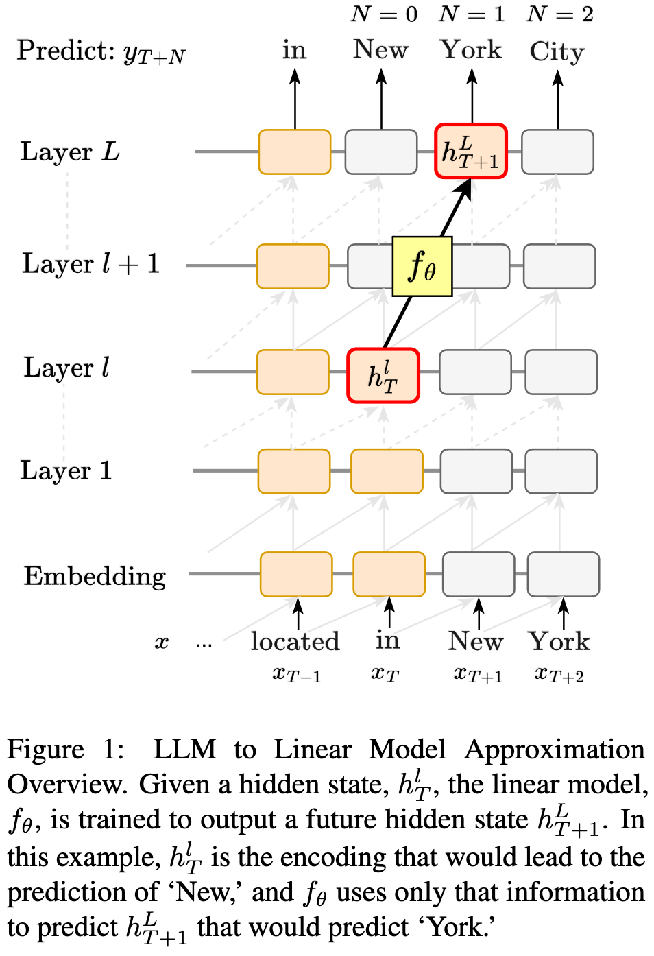
Future Lens: Anticipating Subsequent Tokens from a Single Hidden State
How well can you predict upcoming tokens given only the hidden states for the latest token?
The answer is: kinda sorta well? The last few layers are decent for the next token while the middle layers are a bit better for tokens after that.
I was hoping the answer would be “extremely well,” because that would be promising for skipping or early exiting decoding steps. But if we actually do need the semantics of generating each token serially, that’s a lot harder to speed up.
Transformer Memory as a Differentiable Search Index
Similar to the Neural Corpus Indexer, they just train a model to output the IDs of which docs are relevant instead of having a conventional embedding + search setup.
They manage to get awesome retrieval results out of this, although it’s unclear how the speed vs accuracy curves look.
I’m taking this as more evidence that training a model to spit out document IDs instead of doing conventional retrieval might be promising.
Fast Inner-Product Algorithms and Architectures for Deep Neural Network Accelerators
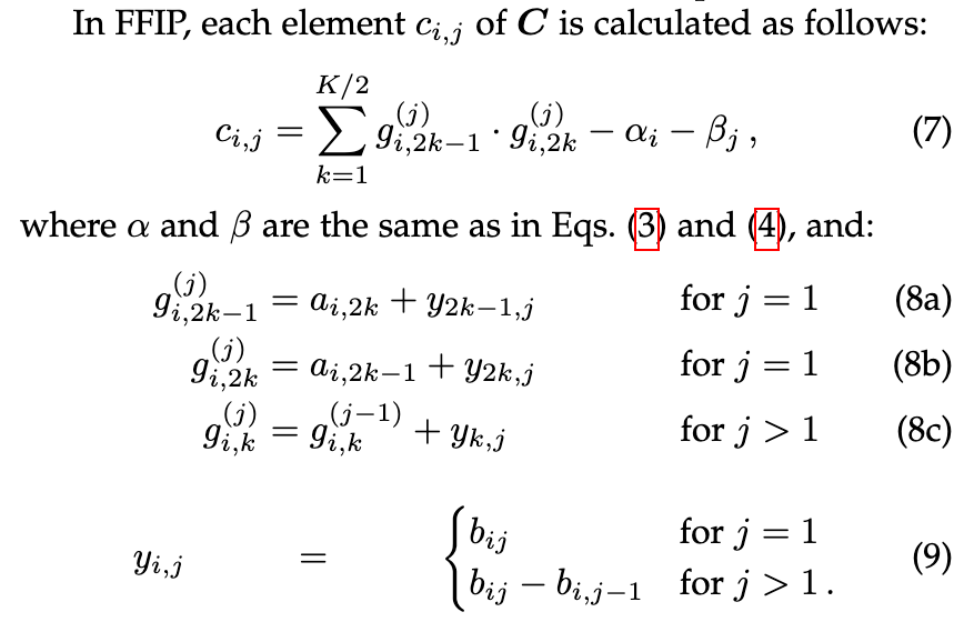
This paper is about computing matrix products with more adds but fewer multiplies, in the same vein as Strassen’s algorithm and Winograd convolution. I don’t understand why the algorithm works, but here it is:
The lets them do an MxN = MxK @ KxN matmul using just (MNK + MK + NK)/2 multiplications instead of the typical MNK multiplications.
They also talk about how this method enables more efficient matmul acceleration in hardware, and how it works well with neural net inference. In the inference case, you can precompute the β_j terms and fuse the b_ij terms into the biases.
I don’t know enough to comment on the hardware aspects, but apparently their method saves a bunch of registers and makes it easy to raise your clock frequency compared to previous approaches.
If future hardware could use 2x fewer multiply units for the same matmul throughput, that would certainly be a big area and power win.
Simplifying Transformer Blocks
They found that you could rip out a bunch of components for BERT models up to 300M params while preserving time-to-accuracy on GLUE. In particular, they remove:
Skip connections
LayerNorms
The projection matrix for the values in the attention
The linear after the attention
They also put the FFN and attention blocks in parallel.
To make this work, they bias the attentions such that the attention module is an identity function during initialization.
Other than that, they evaluate it with essentially the same hparams as a baseline model and find that the time vs loss is a bit better.
I’m surprised they got rid of the values projection matrix instead of either the query or key projections, because the latter two are redundant7. But regardless, these sort of simplifications will be a nice win if others can reproduce them.
I just kinda freehanded all these code snippets, so surely there are some bugs here. But hopefully you get the idea.
It’s definitely the fastest, at least on CPUs. There’s basically no room to output bits any faster unless you ignore the input. What’s unclear is whether it’s provably locality sensitive. I’m like 98% sure it is under reasonable assumptions, but have never gotten around to proving it.
Or at least will go read this literature before gradually reinventing it through an endless stream of subquadratic attention variants. I’m also not 100% certain MADDNESS is still SotA but I’m pretty sure.
That said, the field is identifying a bag of tricks to reduce the accuracy loss:
Approximate layers sequentially and finetune after each approximation
Relax the hard centroid assignment to be differentiable
Finetune for a long time
Don’t replace the first few layers, and possibly the final softmax
Optimize the lookup tables directly, instead of the weights
We can also exploit activation reuse to use more expensive encoding functions, instead of the hash-based one. This could be KV cache reuse, spatial position reuse with K x K filters in a convnet, or feature reuse in a DenseNet.
If you code a binary matmul on a recent CPU, it will get compiled to a bunch of shufb or equivalent table lookup instructions. More generally, xnor + popcount might (?) be a bit lower power than table lookups, but I’d be awfully surprised if it was enough to compensate for the worse space vs accuracy tradeoff.
Shoutout to that time an algorithm that won a Best Paper award offered literally no benefit in the regimes reported, and only appeared better because the baseline was an unoptimized Hugging Face model implementation while their approach used an optimized NVIDIA implementation.
Observe that:
In other words, we gain no expressivity by learning two projection matrices instead of just one. There might be subtle weight decay differences, but adding in extra parameters and FLOPs to preserve poorly-understood regularization interactions is textbook cargo-cult programming and surely not ideal.


