
2023-9 arXiv roundup: A bunch of good ML systems and Empirical science papers

Got behind the curve again and ended up taking me more than a week to catch up. Y’all need to not write so many papers…
Are Emergent Abilities in Large Language Models just In-Context Learning?
They make two claims:
“Emergent” capabilities of LLMs are a consequence of in-context learning (i.e., including some examples in the prompt). If you don’t add in-context examples, the model doesn’t have these capabilities.
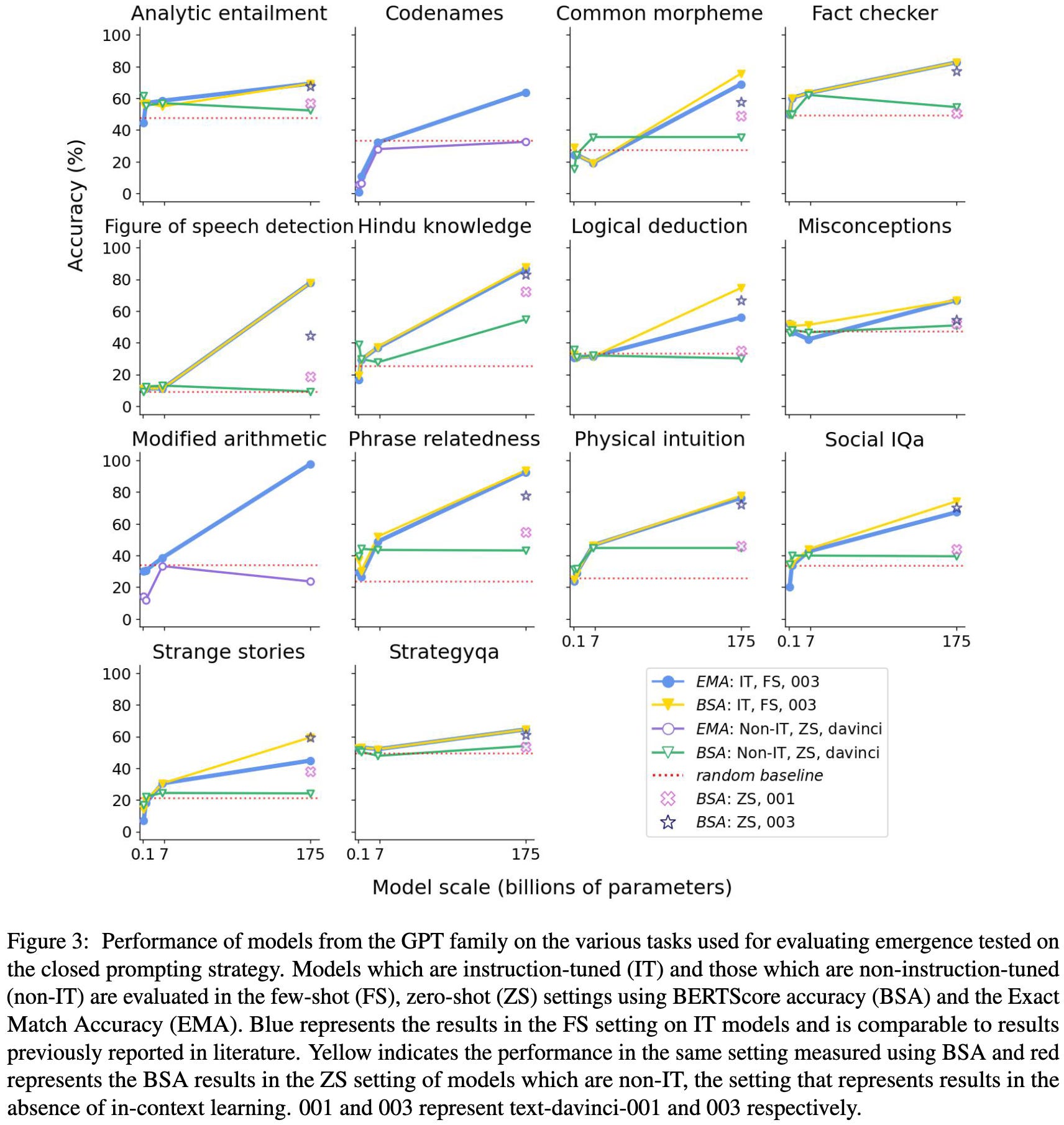
Instruction tuning helps by enabling the model to do in-context learning.

These claims seem to be supported by their experiments.

Probably doesn’t close the book on emergent capabilities, but this is at least a really thorough analysis with a lot of experiments. I’m pretty sold on emergent capabilities being possible on toy tasks where you have to get k independent subproblems right to get the overall answer right (since this would yield exponential final accuracy wrt subproblem accuracy), but this might be a contrived scenario that doesn’t resemble real tasks.
Their conclusions are good news from an AI risk perspective; if almost all capabilities really do show up smoothly (unless you go out of your way to provide demonstrations), we won’t get leaps we weren’t expecting.
Scaling Autoregressive Multi-Modal Models: Pretraining and Instruction Tuning
They generated awesome images with a decoder-only transformer instead of a diffusion model.

A few qualitative aspects that stood out to me:
Decoder-only image generation. Patches are tokens and they generate patches serially.
No dropout or trainable params in the layernorms.
Use of a big Shutterstock dataset that actually respects image licenses
Retrieval augmentation using CLIP embeddings of multimodal documents with some heuristics to improve diversity of the retrieved set
Joint text and image prompting + output


Quantitatively, it offers a much better training compute vs FID tradeoff than existing alternatives.

The models aren’t that big. The biggest one is 7B params trained on 2.4T tokens.

Pretty interesting to see a non-diffusion model work so well for image generation. This might also be the first example I’ve seen of a retrieval-augmented model reporting a better time vs quality tradeoff than a retrieval-free baseline. Highly speculative, but maybe this is easier to achieve when image retrieval is involved, since images give you way more bits of context per retrieved element than text documents do?
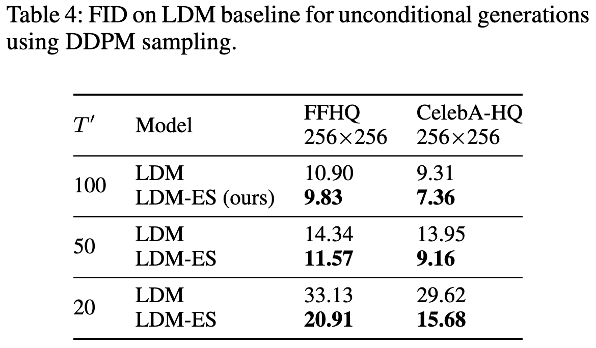
Elucidating the Exposure Bias in Diffusion Models
There’s a train-vs-test discrepancy in the variance of activations of diffusion models across sampling steps, with the test-time variance being significantly larger.

To mitigate this and better align the test-time sampling with the training distribution, they propose Epsilon Scaling, which scales down the activations according to a schedule.

This is apparently a free win across various datasets:


SARATHI: Efficient LLM Inference by Piggybacking Decodes with Chunked Prefills
They do two clever things to improve hardware utilization during LLM inference:
They split up processing of the prompt (“prefill”) into the processing of smaller chunks. This creates uniform units of work that can be batched together across different queries, and helps avoid pipeline bubbles during pipelined inference.
They combine the latest token from autoregressive decoding for one query with the prefill of another query. This lets them do slightly larger matrix products instead of doing separate matrix-vector products (in the batch size 1 case) or matrix * tall matrix products (in the batch size > 1 case).
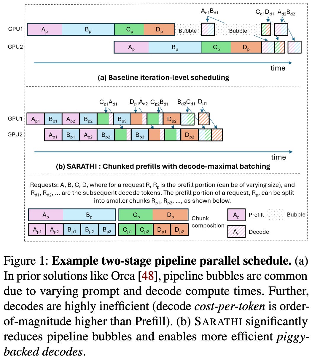
This presumably relies on having some combination of enough queries in flight at once and a high enough ratio1 of prompt length to number of generated tokens. But if you meet these conditions, this seems like a clear win.

Until the prompt length dominates the generation length, this method works better than a strong baseline:
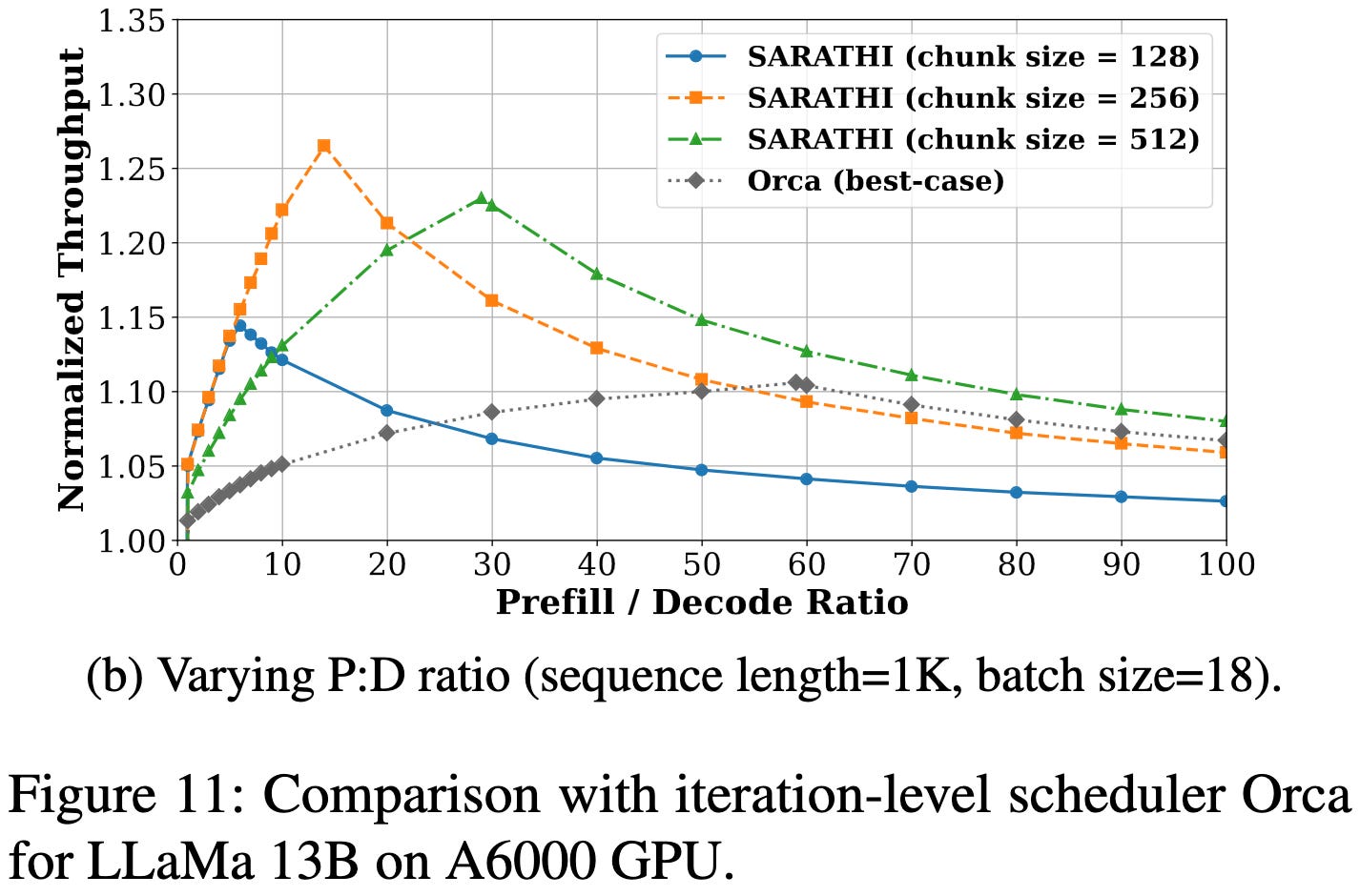
Also, they have a bunch of good plots of profiling results:


I’d have to stare at it longer to be sure, but coalescing the decode matvecs into the prefill matmuls seems like clearly a good idea.
On the Implicit Bias of Adam
Adam penalizes various norms of the gradient depending on the relationships between β1, β2, and ε. Note that ρ in this table is typically called β2.

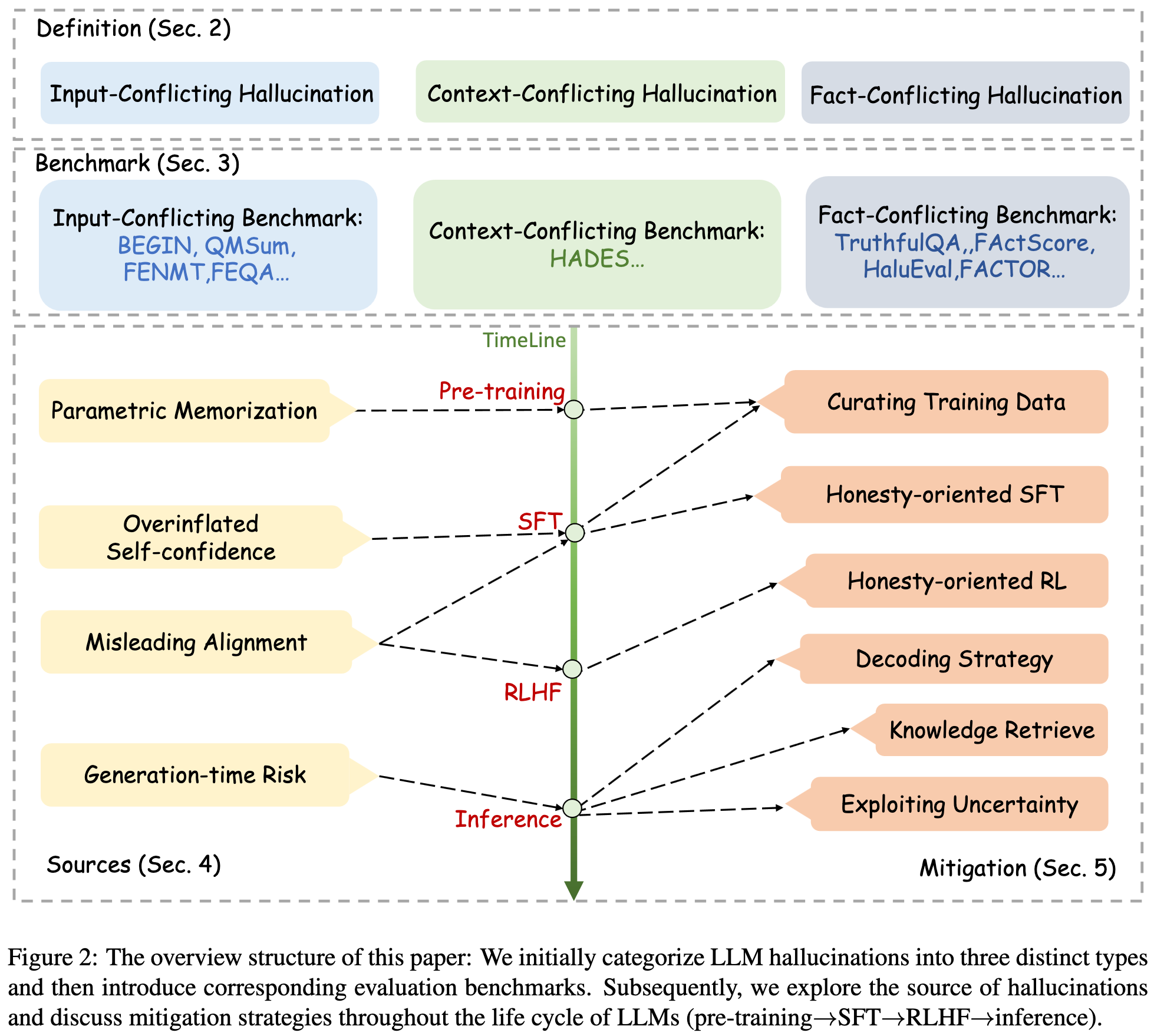
Siren's Song in the AI Ocean: A Survey on Hallucination in Large Language Models
Survey of hallucination in LLMs, including mitigation strategies and benchmarks you can use to measure it.
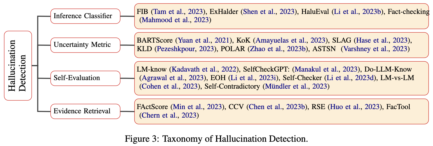
Cognitive Mirage: A Review of Hallucinations in Large Language Models
Another survey of hallucinations.

Memory Efficient Optimizers with 4-bit States
The bad news for me is that I kinda got scooped here (unless pull requests count?). But the good news for you is that I can tell you why at least one part of this is a great idea.
But first, let’s start with the goal: they’re trying to do 4-bit quantization for the two Adam state tensors, which track the first and second moments of the gradients.
They quantize the moving average of the gradients using linear quantization with a block size of 128. This apparently just kinda works.
For the moving average of the gradients squared, they have to do something more interesting2. Instead of splitting the tensor into disjoint chunks and storing the max value in each chunk as a scale factor, they instead store the max value in each row and column. The key is this: the scale factor for a given element is the minimum of its row max and column max. This guarantees that all elements have value at most 1 after scaling, but makes outliers in a given row or column not blow up the scale factors for all their neighbors.

More generally, you can hash the elements to k buckets, store the max of each bucket, and gain robustness to at most k-1 outliers. The downsides of this approach are that it:
increases the size of your stored scales by a factor of k, which isn’t worth it for small enough tensors (e.g., 8x8, or 8x8x8);
complicates your kernels and (for large enough tensors) requires you to hit shared memory instead of keeping everything in registers;
eventually increases the average scale factor you use as k gets large. With iid elements and some math, you can show that the probability of the scale factor for a given element exceeding some value 𝜏 is roughly k*p(𝜏)^k, with the “roughly” coming from a union bound over bags. Here p(𝜏) is the probability that the max of a single bag exceeds 𝜏. So you kind of end up concentrating your scale factors towards a large-ish value but you ensure they’re almost never a huge value.
Besides this approach, they also consider just doing Adafactor and applying regular linear quantization to the factorized moments. This and the multi-bag approach seem to work best.

With the quantization done well, they get away with 4-bit optimizer state tensors without accuracy loss (on average).
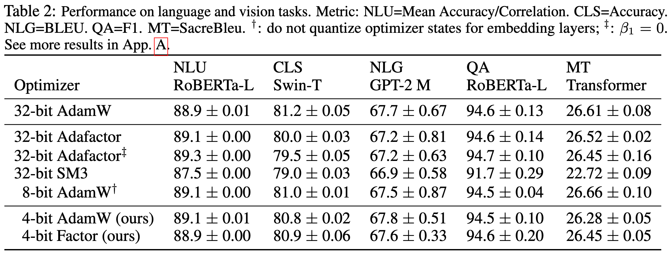
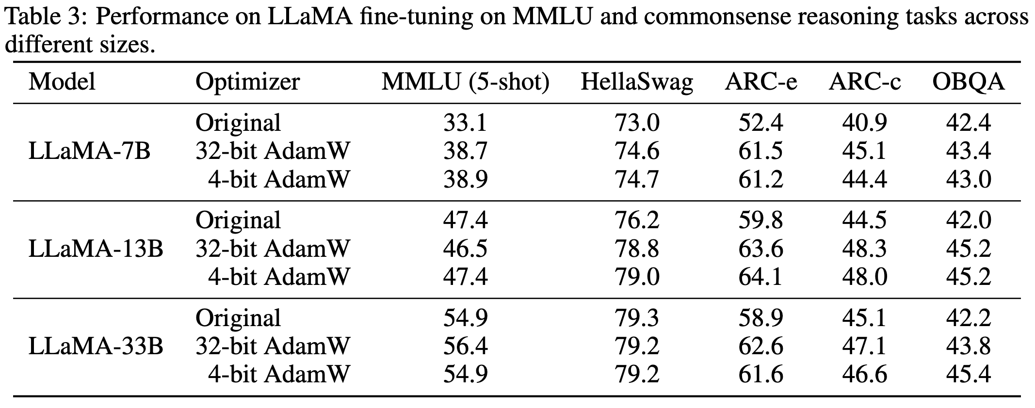
Cool to see 4-bit optimizer states working well. It doesn’t seem completely reliable in preserving accuracy yet, but with more granularity in the quantization block size and good preprocessing, I’d bet you could get there.
Softmax Bias Correction for Quantized Generative Models
Turns out the softmax activations in diffusion models are especially sensitive to quantization. This seems to be because there are so many tiny positive values that all get rounded to zero; this both introduces bias (since more stuff gets rounded down than up) and screws up the sum-to-one property.
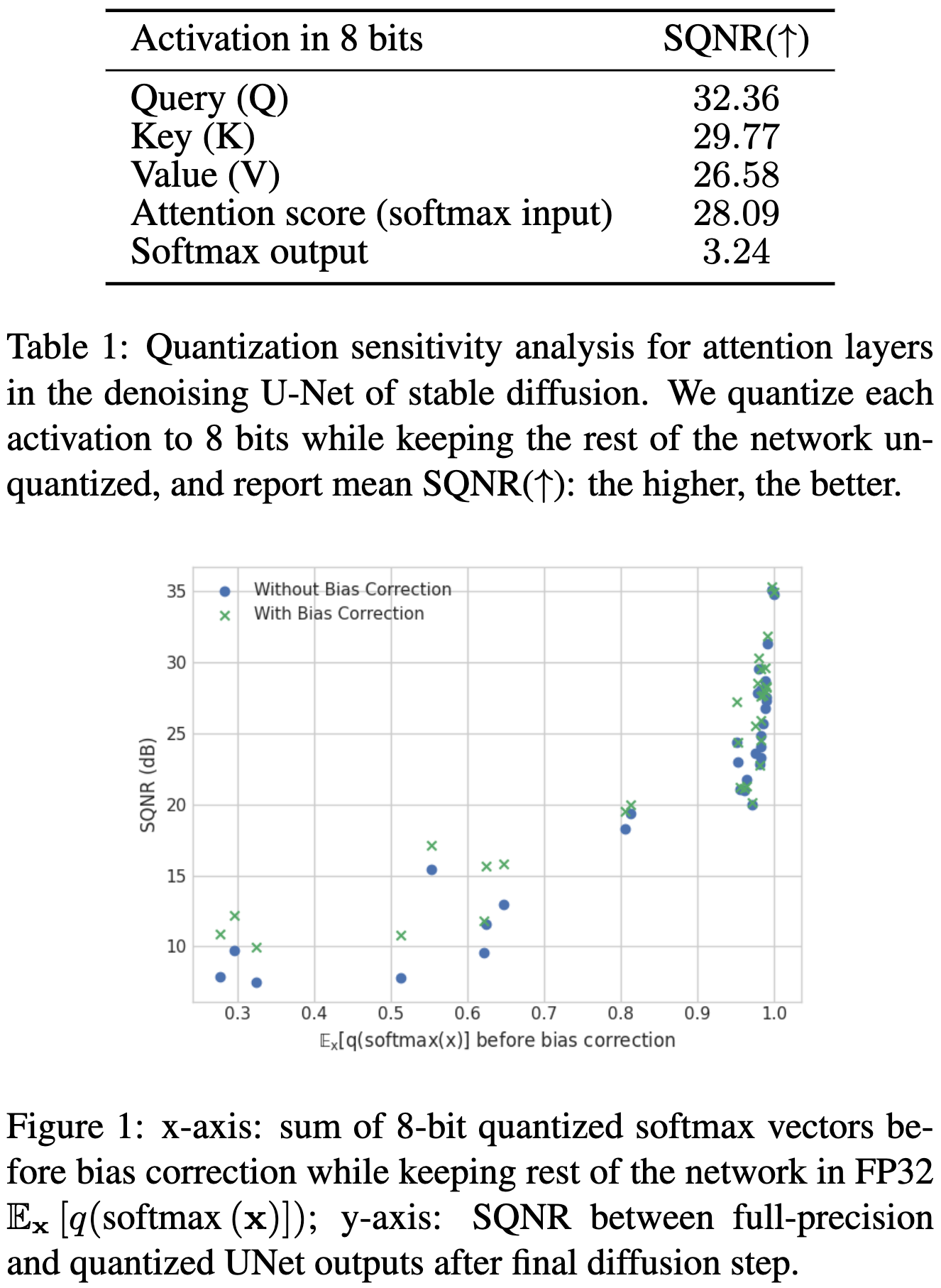
To fix this, they use some calibration data to estimate the bias added per-tensor or per-attention-head. They then add in these correction factors as part of the quantization function.

This correction seems to improve the quality of the quantized model significantly.


Man, Qualcomm’s been killing it as far as empirical analysis of numerical issues lately.
Explaining grokking through circuit efficiency
The authors already have a great summary here, so I’ll just give an even quicker version. Basically, there are two sets of weights to think about:
“Mem,” a point in parameter space that just memorizes the input, and
“Gen,” a point in parameter space that generalizes to new inputs.
Groking happens when:
both of these points exist,
Mem is easier to learn, and
Gen has lower weight norm (and therefore lower effective loss when including weight decay).
This set of conditions causes the network to converge to Mem early in training / for small datasets, but eventually move towards Gen later in training / with bigger datasets. The dataset size matters because memorizing gets harder the bigger the dataset, while finding the generalizing solution (for some problems) is constant difficulty.


Makes a lot of sense, and I’m always a fan of papers that try to figure out the physics rather than optimize the alchemy.
DoLa: Decoding by Contrasting Layers Improves Factuality in Large Language Models
They propose a heuristic for increasing the factuality of language models. The heuristic is based on the idea that later layers are more likely to encode factual knowledge.

Basically they intelligently select an early layer and use the difference in logits between that layer and the output to adjust the token probabilities.

Apparently this heuristic works pretty well, at least on a couple datasets.


Large Language Models as Optimizers
They use LLMs to optimize LLM prompts, as well as to solve other optimization problems.

Here’s an example of how they prompt an LLM to generate a better prompt:

Their optimized prompts can work better than handcrafted prompts. In particular, their method discovers “Take a deep breath and work on this problem step-by-step,” which can yield much higher accuracy than “Let’s think step by step.”

Language Models as Black-Box Optimizers for Vision-Language Models
Similar to the above, they use LLMs to optimize prompts.


The result, at least for image classification with vision + language models, is a dataset-specific template that gets filled in with the class name.

These prompts tend to work better than existing alternatives.

Another example of using ML to improve the results we get from ML.
Mobile V-MoEs: Scaling Down Vision Transformers via Sparse Mixture-of-Experts
An Apple paper trying to get sparse mixture of experts models to fit on iPhones and other resource-constrained devices. They shake up the normal MoE formulation by routing at the image level rather than the patch level, which also couples the routing decisions across all layers.

This buys them the ability to only load a subset of the experts for a given input and do aggressive prefetching. A subtler aspect is that it guarantees a good batch size for each activated expert, since you feed it the whole input instead of a subset of tokens.
They also train the router based on class clusterings, grouping similar classes together within each expert.

It’s not clear how this compares to a typical MoE setup, but it certainly beats a FLOP-matched dense model.

I spent a bunch of time a couple years ago thinking about the most efficient possible MoE formulation from first principles, and it’s basically this (if you can get away with not having causal masking). By bundling many tokens together in your routing decisions, you can simultaneously:
Guarantee that every expert gets enough tokens to run a matmul at decent utilization
Allow limitless experts with zero marginal runtime cost—just extra RAM.
Of course, RAM does matter, and you also will end up undertraining your experts if you have too many of them. But I still think the ability to scale up param count this seamlessly is super interesting from a system design perspective. Maybe we’ll get away with way fewer FLOPs and way more RAM in future accelerators or offload way more params to CPU RAM.
When Less is More: Investigating Data Pruning for Pretraining LLMs at Scale
They experiment with a bunch of different design choices regarding which subsets of your text data to remove before pretraining.

The pruning involves a straightforward scoring of each sequence using some heuristic, followed by discarding sequences based on their scores.

First, they find that you don’t want your chosen subset to just consist of the easiest / most memorized samples.

Whether to keep the bottom, middle, or highest-scoring samples depends on the scoring function and the fraction of samples you’re keeping. Keeping the middle 50% is best with one scoring function (left), while keeping the bottom 70% of samples is best when scoring how memorized the samples are (right).

Just looking at perplexity works at least as well as more sophisticated scoring functions across a variety of subset sizes. Fancier approaches often fail to beat the baseline of not pruning data at all. They keep the samples with the middle perplexities here, discarding both the highest- and lowest-perplexity ones.

For scoring functions that use a reference model, using a model trained on Wikipedia beats using one trained on all of CommonCrawl. Larger reference models also tend to do better, but even undertrained reference models often score samples at least as well as fully trained ones.

Their findings seem to hold even as model size increases.

Really thorough empiricism. Always great when a paper asks an important question and tries to get to the truth rather than sell a particular solution.
SA-Solver: Stochastic Adams Solver for Fast Sampling of Diffusion Models
You can formulate sampling from a diffusion model as solving a differential equation. They use math to formulate this problem as a tractable optimization problem and solve it via alternating prediction + correction steps, instead of just applying the model over and over again.
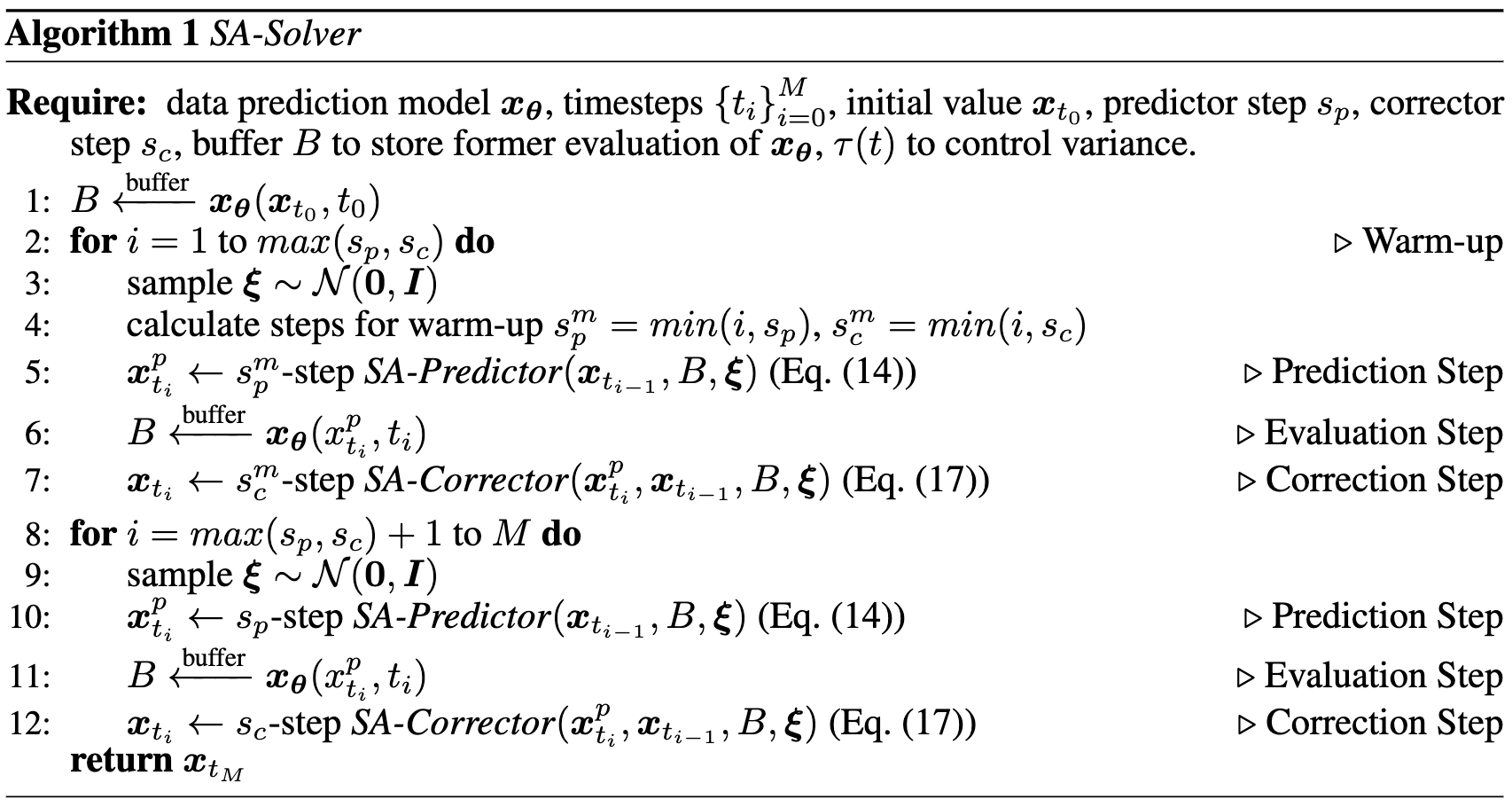

Their algorithm achieves a much better tradeoff between number of diffusion steps (“Number of Function Evaluations”) and FID.


I’d need to stare at this a lot longer to really get what’s going on, but this seems like a large time vs quality win for diffusion models.
Pushing Mixture of Experts to the Limit: Extremely Parameter Efficient MoE for Instruction Tuning
Instead of learning fixed LoRA matrices or featurewise activation scales, they have a bunch of different matrices/scales and dynamically select a linear combination of them based on the input activations.

When holding total parameter count constant or finetuned parameter count constant, this use of dynamic linear functions instead of fixed ones increases accuracy significantly. “MoV” is a “Mixture of Vectors” and “MoLoRA” is a mixture of LoRA matrices.
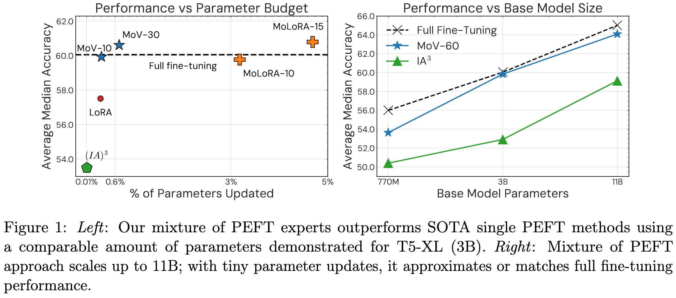

Seems like further validation of dynamic weights being a good idea (esp. if you aren’t measuring wall time), and it’s interesting that you can just add it in during finetuning. Makes me want to try squeeze-and-excitation layers in LLMs.
Efficient Memory Management for Large Language Model Serving with PagedAttention
You want to batch as many requests as possible during inference, but batching too many requests can cause you to run out of memory.

It turns out that a lot of this memory consumption is the result of fragmentation and excessively large memory reservations.

This waste is a natural consequence of how people typically manage KV caches, reserving big, contiguous chunks for each sequence.

They improve memory utilization by splitting RAM into fixed-size blocks and manually allocating + freeing blocks as needed, similar to how virtual memory works.

They can do better than the CUDA or PyTorch allocator because they relax the requirement that the keys and values must be single tensors. Instead, they run a bunch of different matmuls and sum the results. This preserves the math but lets you split up the KV cache into chunks.

This helps them not only avoid excessive reservations for a given query, but also pack the KV caches for different queries into physical memory more effectively.

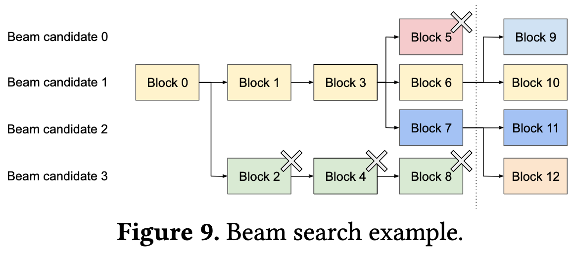
They can use this approach to cleanly handle decoding algorithms like beam search and parallel sampling.

Plus they can deduplicate the KV caches for different sequences with the same prompt.

Their inference runtime, along with some custom kernels, lets them achieve a much better inference latency vs throughput tradeoff than other systems.

A lot of this is thanks to better batching of queries, enabled in part by their memory optimizations.

A well-executed systems paper that seems like just plain the right way to manage KV cache memory.
Scaling Laws for Sparsely-Connected Foundation Models
They look at scaling laws for sparse vision transformers on JFT-4B and sparse T5 models on C4. They make the models sparse by gradually magnitude pruning between 25% and 75% of the way through training.
Their scaling formula adds a coefficient to the number of non-pruned parameters based on the fraction S of weights pruned. More pruning → larger coefficient, since it means that the initial dense network was larger.

This formula fits their observations pretty well, but not so well that I feel like the book is closed on how to reason about sparsity and scaling.

There does seem to be a consistent pattern though of sparser models being better than denser ones by a constant factor across many nonzero parameter counts.

It’s pretty surprising how similar these constant factors are across their T5 and ViT models. Suggests the gains are less of a data distribution thing and more of an architecture and optimization thing.

They also characterized n:m sparsity, since 2:4 sparsity has hardware acceleration on modern NVIDIA GPUs. 2:4 works almost as well as unstructured 50% sparsity, and 4:8 might work even better. 1:4 and 2:8 are much worse than unstructured 75% sparsity though.


One of the most important pruning papers written in a long time IMO, since understanding how sparsity scales is much more impactful than yet another probably-not-better heuristic for how to prune.
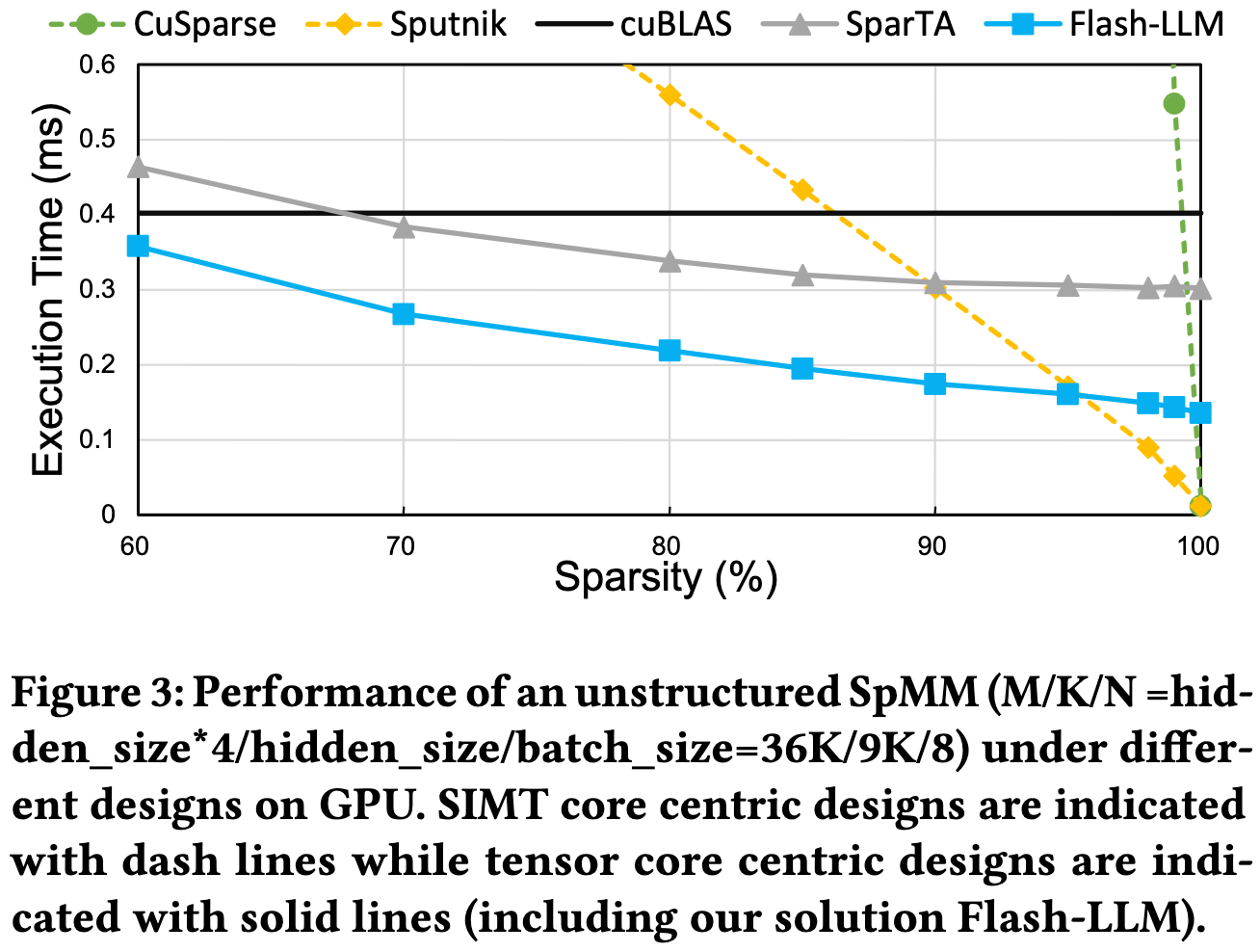
Flash-LLM: Enabling Cost-Effective and Highly-Efficient Large Generative Model Inference with Unstructured Sparsity
They propose to exploit sparsity by just doing sparse loads and not trying to do sparse compute. Instead, they just do dense ops using tensor cores.

Since LLM inference is typically bandwidth-bound, this lets them do faster inference on sparse models.
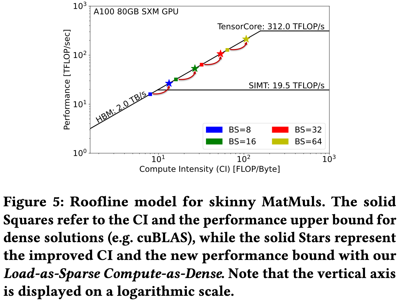
They start running faster than dense kernels at ~60% zeros in the weight matrices, which is lower than other sparse matmul approaches. The tradeoff is that they don’t get to run as fast for extreme levels of sparsity.
Since sparsifying is just one heuristic for making a weight matrix more compressible, this makes me wonder how far we could get formulating the problem more generally. If nothing else, sparsity + quantization should compose fairly well, and would still work with this decompress + dense compute approach (especially since this is the pattern most LLM post-training quantization papers currently use).
The Languini Kitchen: Enabling Language Modelling Research at Different Scales of Compute
This is a long paper, so here are the parts I found most interesting.
First, they do some investigation of what tokenizers are actually learning. In short, there’s a ton of redundancy across tokens, often corresponding to predictable transformations of a fixed word (e.g., uppercase vs lowercase).

Second, they introduce a faster LSTM variant. They give it multiple hidden states (“heads”) and partially unroll the cell state computation along the sequence length dimension. These two changes get it much better utilization on modern accelerators.
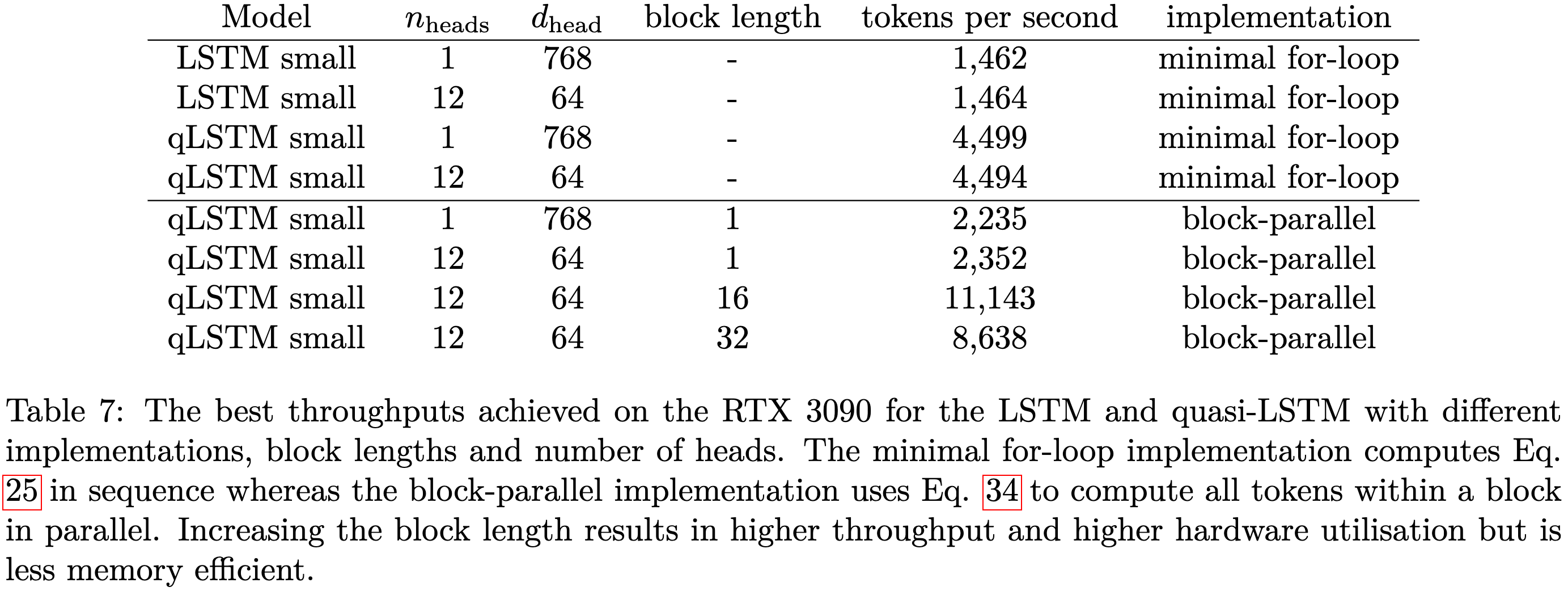
This LSTM variant does significantly worse than a GPT model, but if you linearly extrapolate a few orders of magnitude it looks like it’ll catch up.

I’ve never been sold on LSTMs, but I definitely appreciate the effort to make them work better in practice. And I really like their analysis of tokenizer failure modes.
The Reversal Curse: LLMs trained on "A is B" fail to learn "B is A"
If a model is trained on a sentence of the form “A is B”, it will not automatically generalize to the reverse direction “B is A”. This is the Reversal Curse…
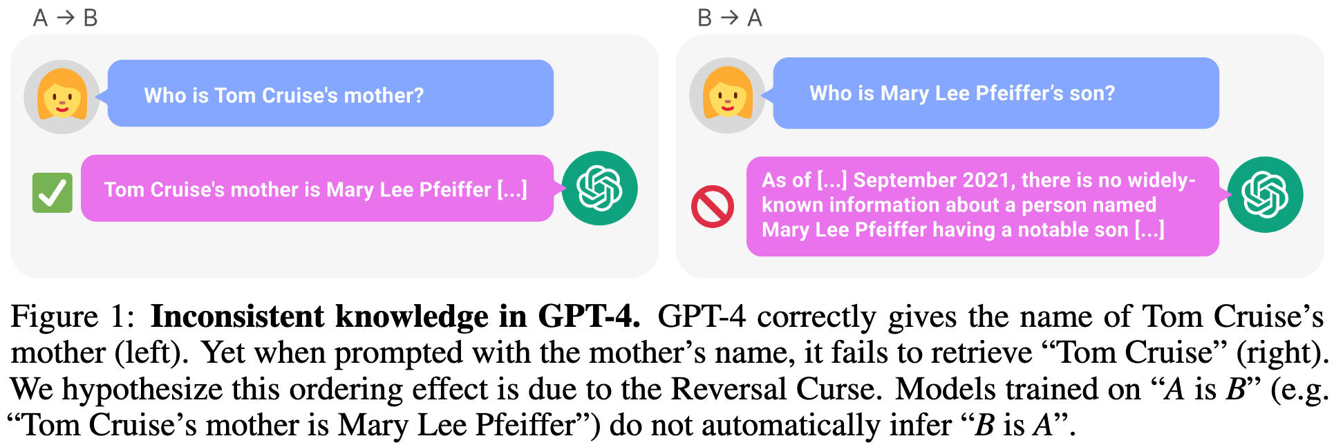
We provide evidence for the Reversal Curse by finetuning GPT-3 and Llama-1 on fictitious statements such as “Uriah Hawthorne is the composer of Abyssal Melodies” and showing that they fail to correctly answer “Who composed Abyssal Melodies?”. The Reversal Curse is robust across model sizes and model families and is not alleviated by data augmentation.

It’s almost like scaling up an autocomplete system doesn’t turn it into a reliable knowledge graph.3
BTLM-3B-8K: 7B Parameter Performance in a 3B Parameter Model
Cerebras trained a 2.6e9 parameter model that yields better outputs than many 7e9 parameter models.
Some design choices that apparently helped:
Training on the “deduplicated SlimPajama dataset”
Using μParametrization
Using ALiBi (instead of RoPE)
Using SwiGLU nonlinearities
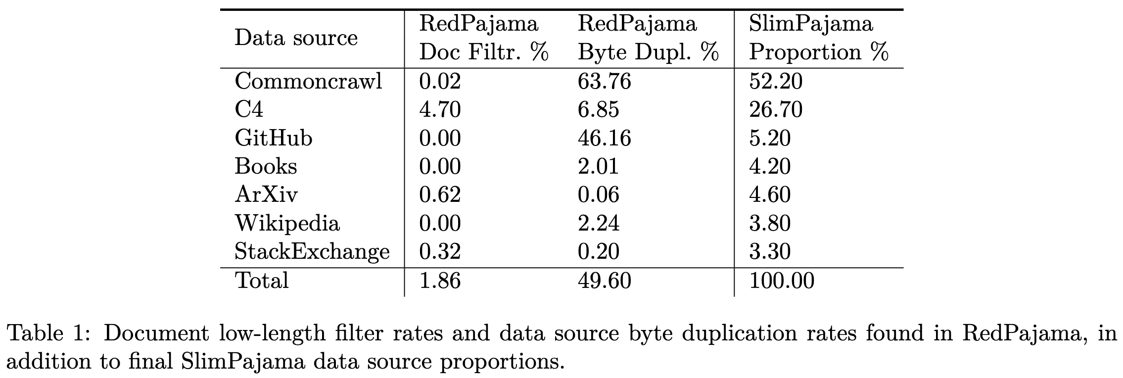
Their data filtering removes docs with <200 characters and docs that are duplicated according to their MinHashes. This rips out ~50% of RedPajama.
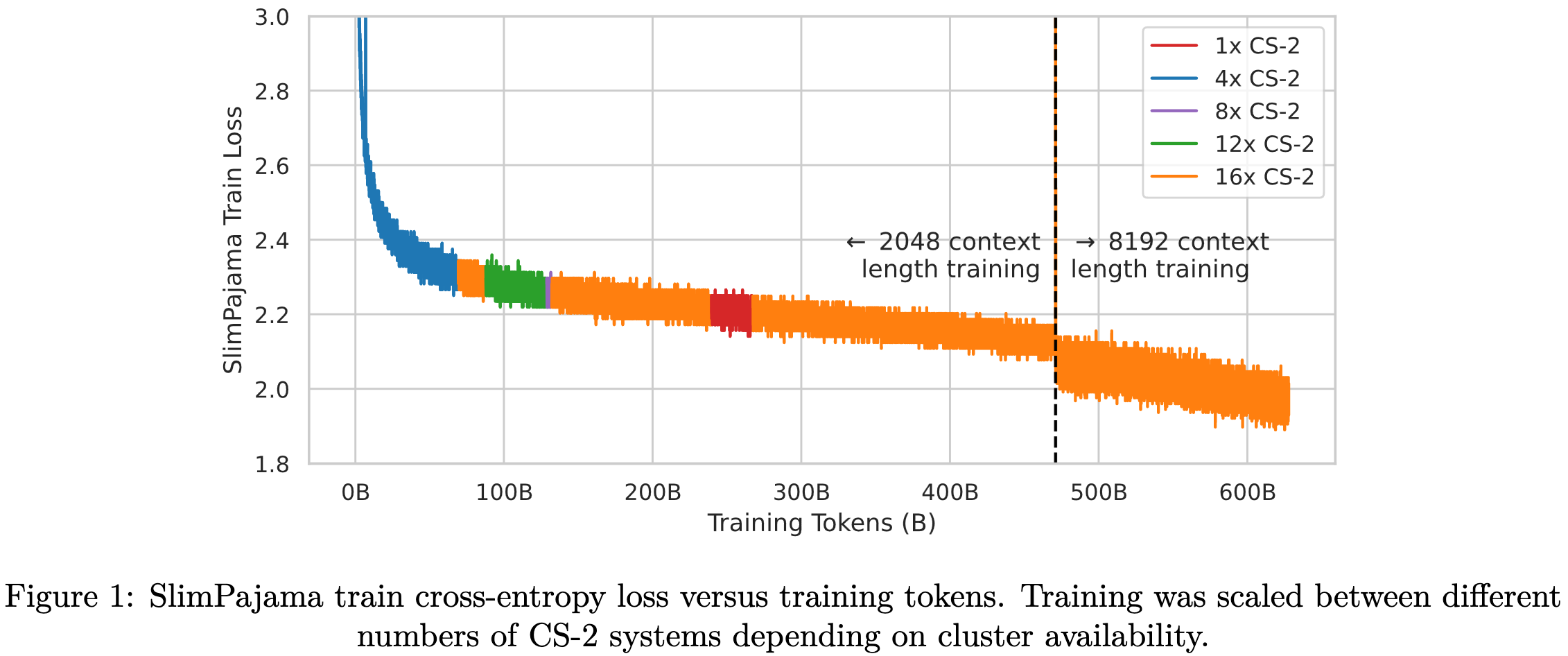
Also, they apparently managed to train it on their hardware, which is pretty cool. I’m not sure I’ve seen any other non-GPU hardware vendors do this with a model of this size and quality.
A useful case study, at least for those of us who care about large-scale LLM training.
LongLoRA: Efficient Fine-tuning of Long-Context Large Language Models
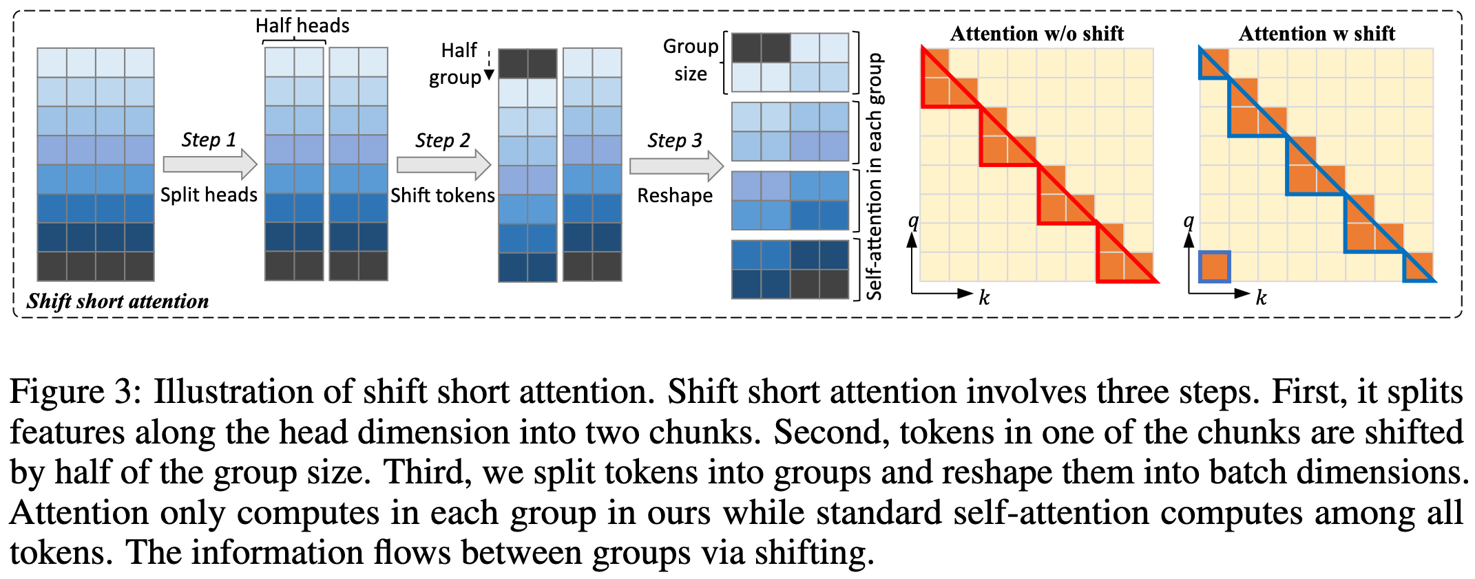
They modify LoRA to train faster and apparently yield better quality when finetuning models to use longer contexts. The weights they train include not just the LoRA matrices for the attention, but also the embedding and norm parameters. They only feed in sequences of the original length during training, but use a more complex attention scheme.

Their attention basically extracts overlapping sliding windows from the longer sequence with a width equal to the original sequence length and a stride of half this width. Each head gets one window and tokens can only attend to other tokens within their window. The last window wraps back around to the start of the sequence.

This apparently works pretty well in terms of peak memory, perplexity, training time, and various downstream eval tasks.

I’m curious whether the window wrapping is an important point; it’s bothered me for a while how it’s hard for outputs to attend to the very beginning of the prompt, so maybe this is an important aspect? It’s also kind of surprising that they got away with having such localized attention otherwise.
Sharpness-Aware Minimization and the Edge of Stability
Neural nets trained with SGD end up at the edge of stability, meaning the curvature of the loss landscape is as large as it can be without diverging for a given effective learning rate. This might be because of increasing curvature as you descend.
For SAM, they find a similar edge of stability result that depends on the SAM step size ρ, the learning rate η, and the norm of the gradients:

I’m not sure what to do with this information but I always like a nice, clean analysis that sheds light on a practical algorithm.
Uncovering Neural Scaling Laws in Molecular Representation Learning
They do a bunch of experiments on scaling neural nets and their training data for molecular stuff.

I was mostly looking at this to see if they found power laws. They did for dataset size.
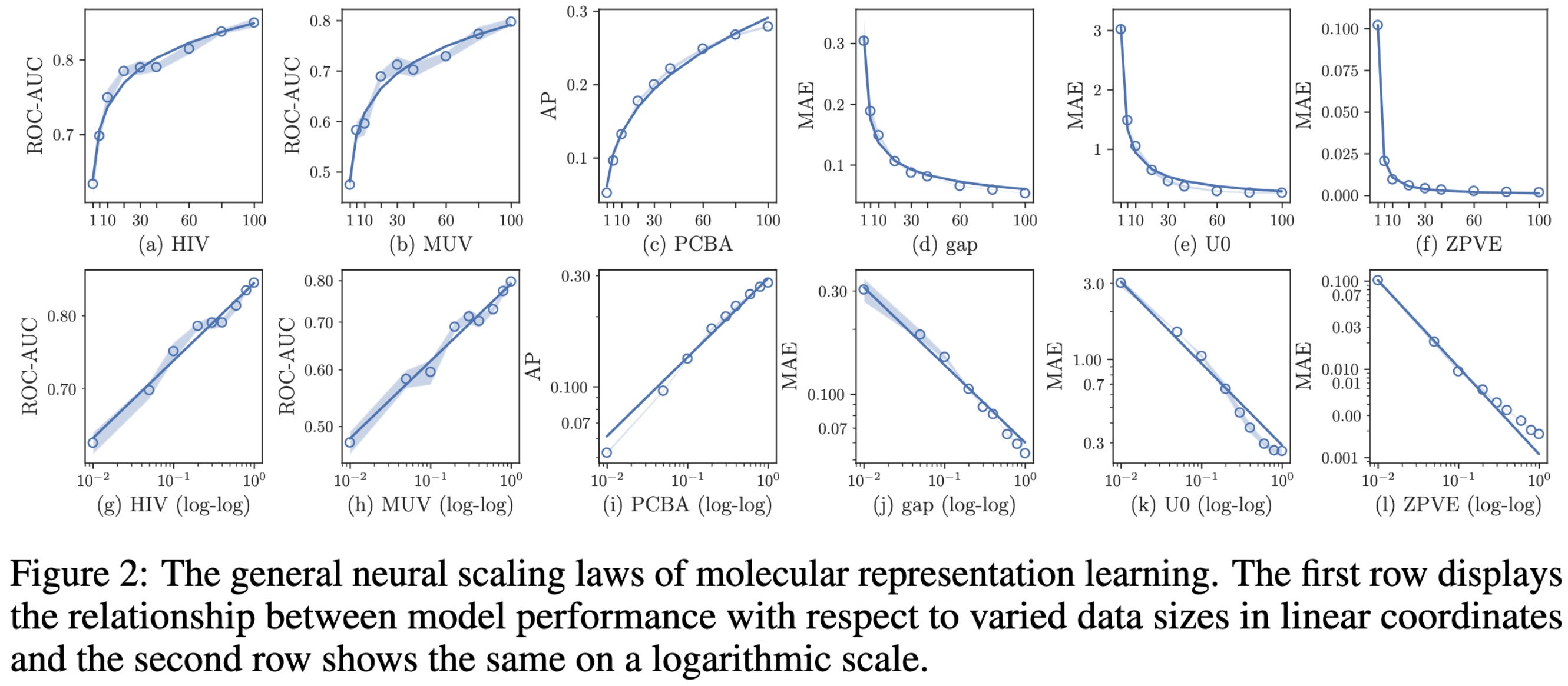
…At least most of the time.

It’s less clear whether they get power laws with respect to MLP parameter count (different curves here are different param counts). Sometimes smaller models do the best, although all of this is at extremely small scale.

Large Language Model Routing with Benchmark Datasets
More evidence that different models have different strengths and you can get an accuracy lift by choosing the right model for your query.


E.g., you can do better than LLama 2 70B by choosing between 13B models, provided you have a few labeled samples and a good scoring function.

Enhancing Sharpness-Aware Optimization Through Variance Suppression
Adding momentum to SAM’s update direction makes it work better.


At least if you tune the momentum coefficient well enough.

The Devil is in the Details: A Deep Dive into the Rabbit Hole of Data Filtering
They investigate a variety of approaches to data filtering for CLIP models.
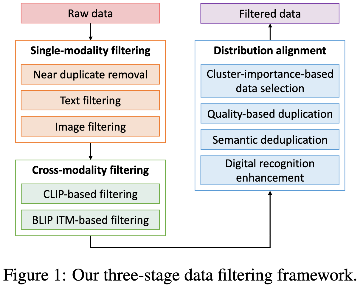
Here’s their summary of what they tried, what worked, and what didn’t work:

It’s only a 4 page paper (excluding apendices) but worth a read if you’re trying to filter an image or text dataset.
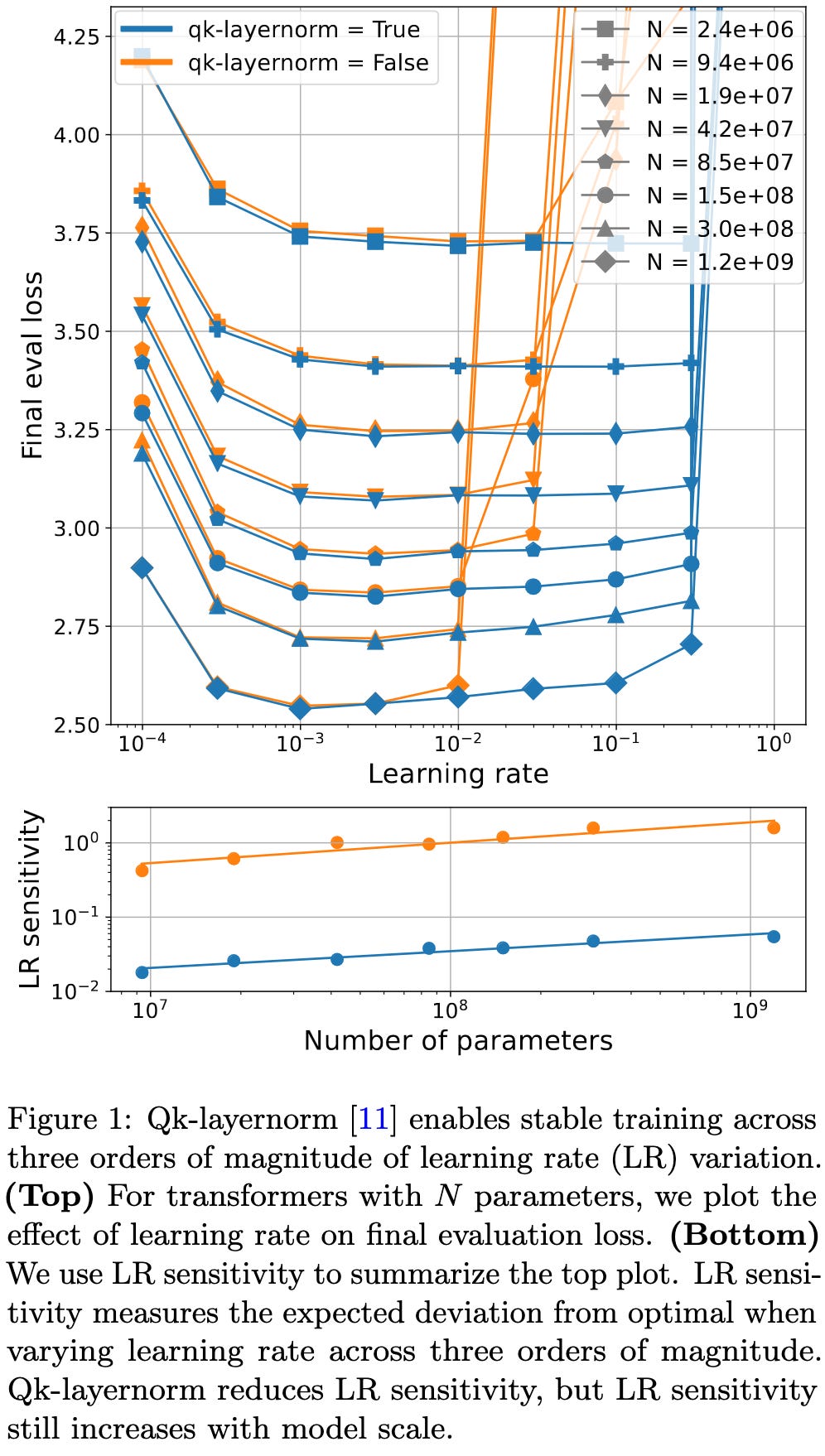
Small-scale proxies for large-scale Transformer training instabilities
They find that they can often replicate instabilities that show up at large scale using small-scale models + high learning rates.

They then use this information to reproduce many claimed instability mitigations. First, QK layernorm (which normalizes the query and key matrices for each head) works great.
The z-loss from the PaLM paper also works. This loss adds an extra loss term of 1e-4 * log(Z)^2, where log(Z) is the “softmax normalizer” at the output layer.

Longer warmup can add stability too.

As can implementing decoupled weight decay properly.

A couple other findings: for one, larger learning rates lead to higher weight norms at fixed weight decay (because math4), which yield larger activations, which yield smaller gradients because of the LayerNorms dividing by the (larger) activation scales in the backwards pass.

A corollary is that, as your learning rate goes up, you might need your Adam epsilon to go down so that it doesn’t shrink the update norms too much.

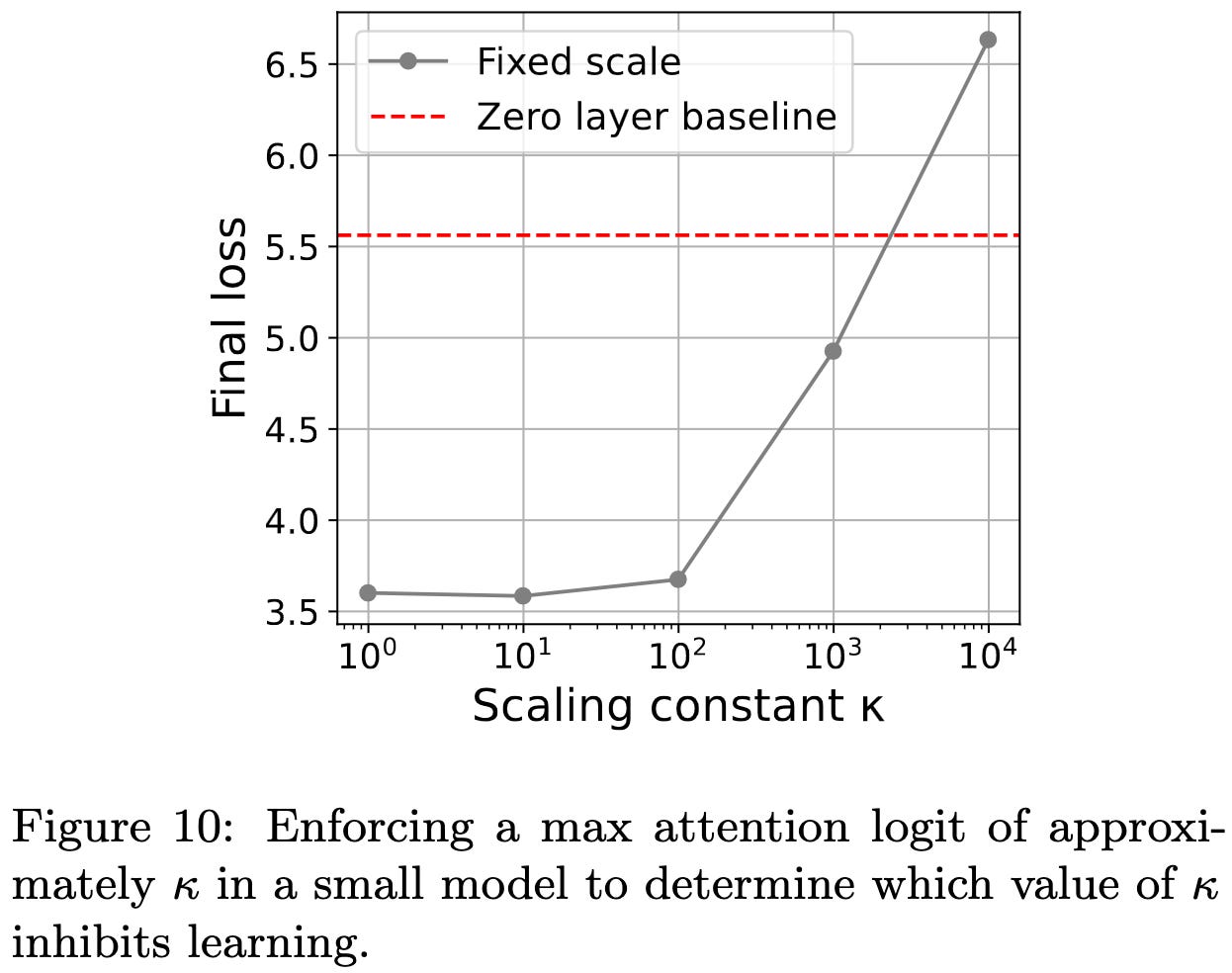
A final standalone result is that you can clip the pre-softmax attention values at 10 without hurting the model quality, at least in the case they tested.
This is a super thorough science-of-deep learning paper and worth a careful read if you care about training stability.
Provably safe systems: the only path to controllable AGI
They argue that AI systems should be proof-carrying code running on “provably compliant hardware” that checks whether actions adhere to a generalized version of smart contracts before performing them.

Since neural networks seem hard to verify, they envision using neural networks to discover scalable algorithms that we can verify.

They also list open research problems whose solutions are needed to make this a reality. As far as this approach being the only path, they argue this based on Godel’s completeness theorem; roughly, any true statement has a proof, so if we can’t find a proof for some safety property, that property might not actually hold and an AGI might exploit it.
On the one hand, I’m all for using formal verification as much as we can when it comes to alignment problems. A formal guarantee is way better than messing around at the reinforcement learning level hoping you somehow incentivize the right behavior.
On the other hand, this is…not how I hear formal verification people talk about verification. Phrases like “provably physically impossible” are just not a thing. You always have some formal model of how the software gets executed, and it’s extraordinarily ambitious to suppose that there will never be any side channel attacks, hardware failures, architecture or language nuances you didn’t model, etc. The physical world and proofs rarely mix; physically unclonable functions are a thing, but I’m personally not aware of other cases of “proof” and “hardware” going together (unless maybe you count trusted execution environments like SGX, but even here you have some root of trust). You also hit the classic verification + alignment problem of needing to provide a spec, which is…difficult even in software, and arguably impossible when considering a general-purpose agent in the physical world.
For perspective on where formal verification currently is, we can do things like verify a network filesystem if you have an expert code the system such that it’s conducive to verification and spend months or years writing the proofs in Coq. I’m hopeful we’ll keep making progress, but given how many decades people have been working on formal verification already, I wouldn’t want to bet too hard on formal verification being “the only path to controllable AGI”—especially if you want a solution in the next decade or two.
That said, it’s great to see an ambitious vision of the future that we can strive towards, and I’m always happy when people publicize formal verification in the AI safety community.
Based on the below figure, you actually get the most benefit for moderate prompt length to generation length ratios. I think this is because the decode gradually stops mattering in this normalized measurement as the prompt length dominates the generation length.
Which is unsurprising given that squaring gradients is absolute numerical madness. Like, if you histogram these tensors, you see that their dynamic range can exceed that of even a float16.
This is me poking fun at insufficiently nuanced takes on “intelligence,” not this paper. The paper does a great job.
More precisely:
Gradients tend to be orthogonal to the weights because curse of dimensionality. If there’s a normalization op right after the weight matrix, this is guaranteed because moving in the direction of the weights just scales the output and therefore has no effect.
But weight decay shrinks the weights.
So if your training doesn’t blow up, you hit an equilibrium norm for each weight matrix. And the larger the learning rate, the greater this equilibrium norm.