2024-8-25: Scaling curves for All of the Things

Good news: we got a bunch of important findings this week.
Bad news: 40+ hours of work and 40+ hours of baby stuff doesn’t leave much time for papers, so we’ve got a shorter installment this week that’s more of a highlight reel.

---

Scaling LLM Test-Time Compute Optimally can be More Effective than Scaling Model Parameters

You know how there are a bunch of ways to get better results out of a fixed LLM by throwing more compute at the inference (e.g., majority voting across multiple generations)? This paper asks the question, “How well can you get your output quality to scale with various approaches to test-time computation?” And in particular, can we beat big models with small models and more complex inference techniques?

You can’t test every possible approach to test-time compute, so they split them into two buckets and sample representative approaches from each. The buckets are:

1. improving the proposal distribution (sampling from the model) and

2. improving the “verifier” that aggregates different outputs.

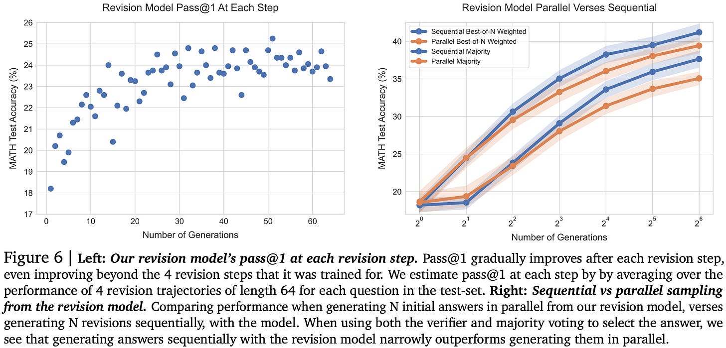
The representative approaches they choose for improving the proposal distribution are sampling multiple responses in parallel vs training a model to iteratively refine the previous output. They also try combinations of both.

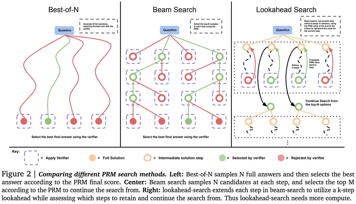
The representative approaches for aggregating outputs are weighted voting, beam search, and lookahead search (which subsumes beam search as a special case and resembles derandomized MCTS). All of these lean on a trained reward model to score outputs; the voting uses it to weight votes while the latter two use it to score nodes in the search tree.

When trying to improve the proposal distribution, you want to optimize your mix of sequential output revisions and parallel generations (local maxima within a line or group of bars, below). But even if you don’t, throwing more compute at the problem consistently helps.

This need for a balance makes sense because they find that you eventually get extreme diminishing returns from more steps of refinement, with correct answers getting broken about as often as incorrect ones get fixed.

When trying to aggregate responses, you usually do the best with a simple beam search. Although at high numbers of test-time generations, weighted voting starts winning. It matters less what you use for easy math problems than for harder ones (right subplot).

If you choose the best test-time strategy based on your generation budget and a learned estimate of how hard the problem is, you can do better than any individual technique.

Also, using a Process Reward Model (PRM) works better than a simple Outcome Reward Model (ORM)—which makes sense given that it’s being used to score intermediate nodes in a search tree.

So now that we’ve learned a lot about what works to scale up test-time compute, how does their most effective test-time scaling compare to scaling up pretraining?

Well…it’s a little complicated. In the figures below, the x-axis is always compute, with 3 pretraining FLOPs exchangeable for 1 inference FLOP (because of the backward pass). The dotted lines are the combined FLOPs for just using a bigger model, with different lines for different ratios of pretraining to inference tokens. The stars on the dotted lines are the bigger model’s accuracy for a given difficulty bucket and token ratio. So basically, if the stars are above the line of the same color, just pretraining a bigger model beats using more test-time compute.

The takeaway here is roughly that you can replace parameters with inference flops for easy math problems but not hard ones. There’s also a trend where huge amounts of test-time compute start beating the larger parameter count, but it’s a more complex story because they used a single, larger model here and really you’d want to scale up your param and pretraining token counts differently for different regimes.

This paper was great in that it changed my thinking about what works and where we’re headed in multiple ways:

1. Simple strategies like weighted voting just keep getting better as you scale up test-time compute. Reliable improvements from simple techniques are a giant neon sign for big tech companies saying “invest more in me!” and I suspect that’s what we’ll see. This is especially likely because, based on eyeballing the plots, the diminishing returns don’t look at flat as the Chinchilla power laws (note that the y-axes are not log scale).

2. There’s a regime where you’re limited by your ability to recognize a good solution, not your ability to generate one. This regime is the core of why synthetic data works and doesn’t violate the information processing inequality. And now we’re seeing this pattern emerge for inference in general, not just inference to produce synthetic data.

3. In case it wasn’t clear from the amount of synthetic data in the Llama 3.1 paper, the ratio of test-time to training-time compute demand is increasing.

4. Batch size 1 inference is becoming a less important workload. We’ve put a lot of effort into clever band-aids like speculative decoding, but the future might just be best-of-k parallel generations as standard practice for many problems.

5. Tree search with Process Reward Models is a legit strategy that people have independently replicated.

6. Many simple models may be replaced with compound systems consisting of proposer and verifier modules that can be trained and improved separately. I’m sure developers will still do the simplest possible thing in many cases, but I could see “train or prompt engineer a verifier” joining the standard bag of techniques like “add RAG,” “finetune on my data,” “stick some examples in the prompt,” etc.

Of course, the above extrapolates quite a bit from a set of experiments that focus just on math problems—especially since math is unusually conducive to having a verifier. But this is how I now see the trajectories we’re on.

---

Large Language Monkeys: Scaling Inference Compute with Repeated Sampling

Another Google paper about scaling up test-time compute. This one also examines code datasets, not just math.

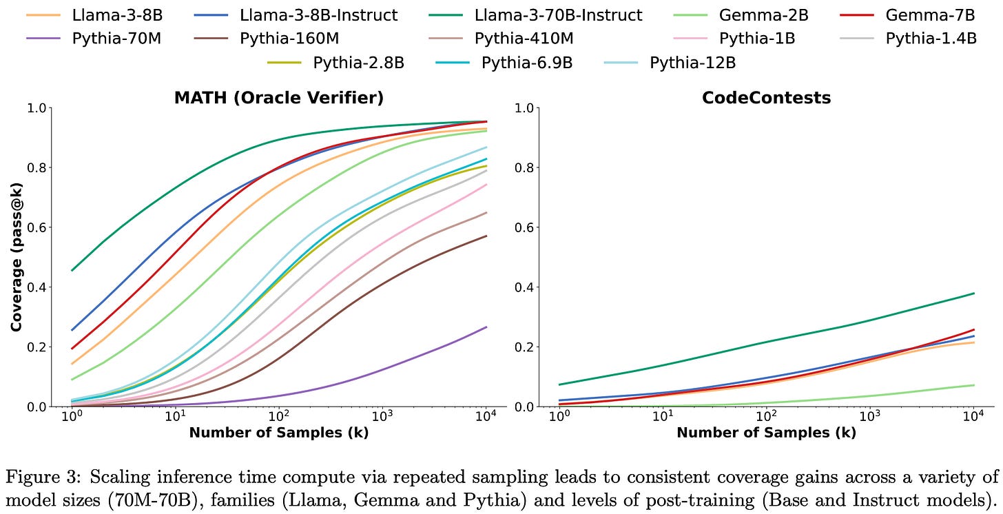
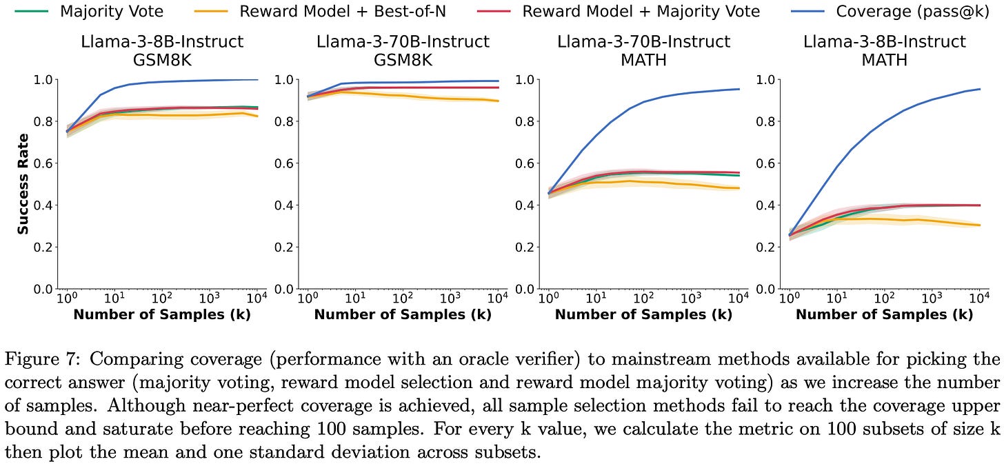
Across a variety of coding tasks, they find that sampling more generations keeps increasing the probability of at least one generation solving the problem. This is not surprising for small numbers of generations, but it’s not obvious a priori that this would keep helping even at 10000+ generations.

They also find that whether you should use a smaller model with more generations or a bigger model depends on the task.

In some cases, using a smaller model + more attempts can work better than using a big, state-of-the-art model. A cool example of this is using DeepSeek’s code model to solve simple (but real!) GitHub issues in 5 attempts instead of Claude or GPT-4o in 1 attempt.

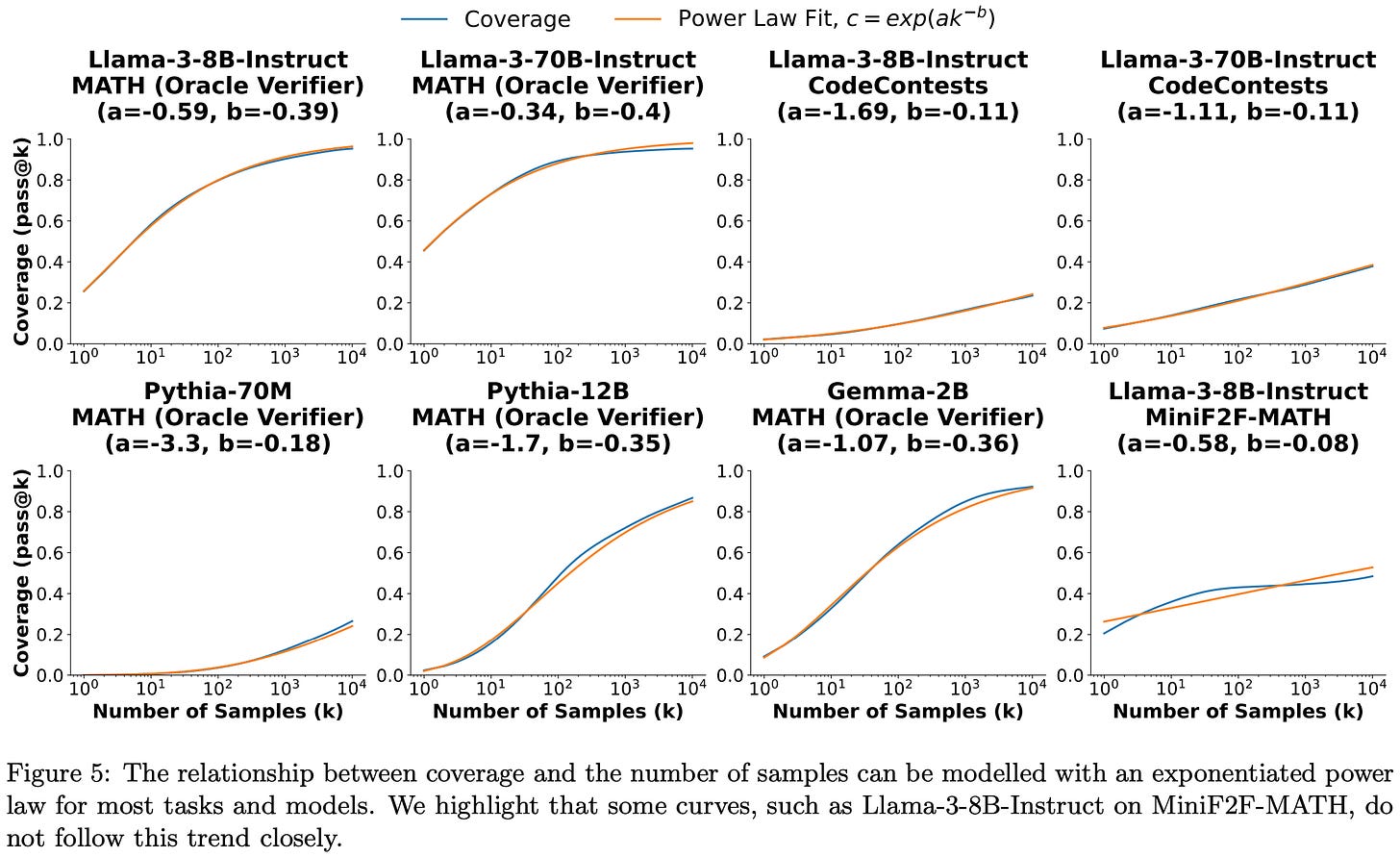
The holy grail here though is finding a clean scaling formula that lets you predict the benefits of any given amount of test-time compute. They sort of find this.

The quality of the fit depends on the model and task, but it looks like the probability of not generating any correct solutions decays exponentially with the number of generations.

This is almost really intuitive; with fixed probability p of generating the right answer, we have a negative binomial distribution and probability 1 - (1-p)^k of generating at least 1 right answer in k attempts. But what’s weird here is that it’s not just exp(constant * k). It uses a power of k instead. I’m not sure what to make of this; I’m pretty sure the generations are iid, so you can’t really get this to happen on a per-problem basis. I’m therefore reading this as a statement about the distribution of difficulty across problems in the dataset.

An interesting related finding is that different families of models have different pass@k scaling curve shapes. So you might not get a some perfect, universal formula, but you can at least estimate large-scale behavior from smaller-scale experiments.

The final result I’ll highlight here is that choosing the correct answer from all the generations is hard. Even in cases like math and code where you nominally have a way to check answers, you often get incorrect tests or evaluation code.

My takeaways from this paper are similar to those from the previous one, so I won’t repeat them. But it’s super nice to see two independent teams replicating the same high-level findings, and even better than they’re doing so on somewhat different tasks and datasets.¹

---

Are More LLM Calls All You Need? Towards Scaling Laws of Compound Inference Systems

They find that aggregating more LLM outputs to make a final prediction sometimes makes the predictions worse after a certain number of outputs.

The reason this happens is that some problems are easy and some problems are hard. Aggregating more outputs is always better for easy problems, but often worse for hard problems. Once you’ve maxed out your chances of getting all the easy questions right for a given dataset, you get a regime change where the decreasing probability of getting the hard questions right takes over.

The way I’m thinking about this is that voting reduces the variance of the estimator, which helps when your probability of being right is >50% but hurts when it’s <50%. More votes means you never get unlucky missing something you should have gotten right, but also never get lucky getting something you should have gotten wrong. Worst case, you have bimodal questions with either a 99.99% to get it right or a 49% chance to get it right, so that reducing variance only costs you good luck and not bad luck.

So how do we reconcile these results with the above two papers finding monotonic scaling, or even closed-form scaling formulas?

The key seems to be the choice of aggregation methods. This paper uses simple (filtered) majority voting, which the other papers also found to not scale as well as alternatives.

That said, I buy their theoretical analysis since it leans on simple assumptions. So I would expect that it’s possible to get non-monotonic scaling under some circumstances even with fancier reward-model-based aggregation functions. And even if it’s not, this paper gave me clearer thinking about ensembling.

It’s also encouraging to see independent empirical and theoretical evidence that sample difficulty is a key factor to look at when reasoning about test-time computation.

---

When Scaling Meets LLM Finetuning: The Effect of Data, Model and Finetuning Method

To what extent to different factors, like model size or finetuning dataset size, affect the quality of your finetuned model?

To answer this question, they did a ton of experiments on 1-16B param LLMs for various multilingual tasks with various finetuning methods.

First, finetuned model quality is more sensitive to model size than finetuning dataset size. This holds across full model tuning (FMT), prompt tuning, and LoRA. I’m reading this as more evidence for the superficial alignment hypothesis.

Same goes for the finding that pretraining dataset size matters more than finetuning dataset size (note that the rightmost subplots are constant because they don’t do any finetuning):

But even finetuning dataset size matters way more than the number of parameters added by your PEFT method. This makes sense since LoRA and prompt tuning add so few params relative to the size of the original model.

Overall, they manage to fit power law curves to these findings with minimal error even on held-out scaling configurations.

Although the coefficients in the formula vary by finetuning and method and task. Ideally, you’d like some universal constants that let you avoid curve fitting on new problems—but I would be shocked if real-world data admitted such a clean shortcut.

There’s a ton of detail in this paper and it’s worth staring at thoroughly if you care a lot about finetuning. There are always question marks around how well the findings generalize to other problems, downstream metrics, etc, but sweeping this many {finetuning methods x model sizes x pretraining data sizes x finetuning data sizes} is already unusually comprehensive and a great contribution.

---

Scaling Law with Learning Rate Annealing

So you know how we have power law scaling curves to let you estimate the final loss for an LLM training run given a bunch of other, smaller runs?

What would be even better is if we had a formula that also predicted loss within a training run, taking into account the learning rate schedule. Besides letting us save a lot of compute by predicting the outcomes of training runs early, this would also shed light on what design choices actually matter in a learning rate schedule.

We now have such a formula:

Let’s break down what this says and discuss what they do and don’t demonstrate. The core claim is that the learning rate schedule can be characterized by two constants: the area under the schedule (S1) and the sum of the momentums of decreases in the learning rate (S2).

The S2 term is the weird one and makes more sense when you think of it as an integrated exponential moving average (EMA) of learning rate decreases. This says that bigger, earlier drops reduce the final loss more.

They arrived at this EMA formula based on empirical observations of the relationship between learning rate and loss. The loss follows the learning rate (including increases!), but with a small, setup-specific delay.

I saw this same relationship of learning rate driving quality in our cyclic learning rates paper, but I’m actually not sure if we saw the delay. The raw loss curves are lost to time/account migrations, but I don’t think we saw it with downstream metrics (part of our Figure 1 clipped below:)

But regardless, this observed lag between learning rate changes and loss changes is what motivates their use of learning rate momentum in their formula.

So how well does this formula work? It’s not perfect but it’s pretty good, even on funky learning rate schedules.

It also plays nicely with parameter and dataset size scaling if you just add the classic power law terms for those features.

In principle, this means that you could fit your parameter and dataset size scaling coefficients based on just one or two runs, using each run to collect many samples instead of just the final loss.

When they try this though, they get way a worse scaling exponent than the Chinchilla paper (~.21 instead of ~.34). But it’s unclear if this is a result of the training setup or the proposed sampling of multiple points per curve.

One impressive aspect of their results is that they fit their coefficients not on the whole training curve, or even a prefix of the training curve, but on entirely separate training curves. They fit their parameters on loss curves that used simple learning rate schedules and generalize from there to other schedules.

As an aside, they have an interesting result showing that gradient norms end up proportional to learning rate. You might expect the updates to be proportional to the LR since the LR is, you know, multiplied in at the end. But the gradients growing with LR is not obvious. I think (?) this suggests nearly-constant curvature in the update directions, so that the mapping of step size to change in gradient norm is fixed.

Back to the main results, their reduction of learning rate schedules to a couple statistics and a simple formula has a lot of explanatory power. In fact, they have 8 straight subsections describing how they explain observed phenomenon related to learning rate schedules.

This is really cool, and exactly the kind of work we need more of as a field. Getting something resembling Maxwell’s equations for deep learning is one of the most important problems we have, and this paper—assuming it replicates—looks like a big chunk of progress on this front.

And I mean a big chunk—we’ve gone decades without a good model for how learning rate schedules work and proposed dozens if not hundreds of schedules, and this paper just comes along and unifies seemingly all of it with two terms and four free parameters.

That said, I don’t think this is the last word on the problem. First, as they point out, their formula is game-able in a way that you wouldn’t expect if we’ve fully nailed the “physics” of learning rate schedules.

First, running steps with a learning rate of 0 still decreases their predicted loss (though note that they propose a variant to mitigate this). Second, if I’m thinking through it correctly, the best learning rate schedule according to their formula should be just the highest LR that doesn’t diverge for most of training followed by an instant drop to ~0. Maybe this actually is better, but the ubiquity of smooth decreases makes me skeptical of rewarding sudden plummets. Finally, I can’t tell how good a fit we should expect from just extracting some sensible features from a learning rate time series and fitting some parameters to them—if there are lots of ways to do this with just as good an R^2 value, then it’s less likely that this formula reflects some underlying physics of neural net training.

So I’d be surprised if we all end up using this exact formula to fit training curves—but now that this paper has shown that such fits are possible, I do expect some extremely similar formula to become standard practice.

---

1. Also, in case you’re tempted to read too much into me writing more about one of these test-time compute papers than the others (or take me too seriously as a commentator in general), be advised that the order in which they appear in this installment is just the order in which I happened to open tabs for them.