Have we hit a statistical wall in LLM scaling? - 2023-6-18 arXiv roundup

This newsletter made possible by MosaicML.

---

Tune As You Scale: Hyperparameter Optimization For Compute Efficient Training

I don’t usually care much about hparam optimization algorithms, but this one has some really interesting findings regarding model + data scaling.

The core of the method isn’t super different from other HPO algorithms; they fit Gaussian processes to the hparams seen so far and their resulting metrics. Metrics here include the compute cost, a model quality metric, and an estimate of the best quality attainable at a given cost.

What’s cool is that they bake in the notion of a Pareto frontier, keeping track of which hparam settings lead to the best quality at a given cost and biasing sampling towards this frontier.

They also tailor the method to large-scale model training in various ways. E.g., they downweight settings are likely to OOM and never sample settings that will take too long to evaluate.

In terms of results, their method seems to work really well. On a reinforcement learning task, using it to tune the hparams lets them improve on the state of the art by a ton.

It also seems to do at least as well as other hparam tuning algorithms across a few different tasks.

But two findings stood out to me. The first was the presence of some non-obvious trends regarding architectural hparams. They found that as your training budget increases, you should scale up the FFN width, number of layers, and number of attention heads, but scale down the QKV feature dimensions.

But here’s the result that really got my attention: they reproduced the Chinchilla scaling curves just by looking at the Pareto frontier their method discovered.

It’s always cool to see an independent reproduction of a key result in the field. But this is extra interesting because they didn’t just tune model size and training tokens, the variables normally in the scaling formula; they tuned “19 different parameters including regularization terms, schedule, model size and token count.”

And despite this, they still got the same numbers. They also trained for 64 * 35 = 2240 A100-days with each training run capped at 40 A100-days, suggesting they had enough time to exploit these extra degrees of freedom.

The fact that they got nearly identical scaling even when optimizing other hparams suggests the Chinchilla scaling coefficients might be a statistical wall.¹ Like in the same way that you just can’t estimate a mean with error less than O(1/sqrt(num_samples)), it could be the case that you can’t train a decoder-only transformer (or any transformer? or any next-token predictor?) with better power law coefficients.²

It’s probably too early to conclude we’ve found such a wall and there are certainly claims that we haven’t, but if there exist fundamental statistical limits for text models, that has tons of implications for AI moats, timelines, and takeoff speeds. It’s a different world when there are upper bounds on how much scale can help vs when some breakthrough might let us use 10x fewer parameters or samples overnight.

---

---

SqueezeLLM: Dense-and-Sparse Quantization

They got probably the best results so far for 3-bit and 4-bit post-training quantization of LLMs.

Before getting to the method, they do some characterization of their workload. They start with some profiling to demonstrate that the bottleneck for single-sequence inference is reading weight memory. Also, the FFNs are way more expensive than the attention ops, and even the attention op itself is mostly slowed down by the matmul at the end.

They then characterize the distributions of the weights they’re trying to quantize. Consistently across layers, the largest 1/10000th of the weights are 5-10x larger than even the 99.99th percentile weights.

With these observations in mind, let’s look at how they do the quantization. First, they allow their quantization bins to be non-uniform. This basically means you find your bin centroids using k-means instead of spacing them uniformly. But instead of weighting all the parameters equally in the centroid update, they weight them based on an estimate of how sensitive the network is to their values.

This sensitivity estimate is the diagonal of the empirical Fisher Information Matrix, which I believe (?) is just the gradient elementwise-squared.

The second component is pulling out the outlier weights into a separate sparse matrix and decomposing the matmul into the sum of a quantized dense matmul and an fp16 sparse matmul. Outliers are defined by either high magnitude or high sensitivity.

To make this sparse + dense sum efficient, they have some interesting kernels that fuse the two operations. These kernels also do part of the sparse matmul as dense operations since they found that certain features are so likely to have nonzeros that it’s worth it.

Putting the sensitivity-based quantization, outlier handling, and efficient kernels together, they get what are likely the best quantization results reported so far for LLaMA models,

as well as Vicuna models.

Their method doesn’t run quite as fast as at least one baseline, but I’m guessing it still yields a better Pareto frontier based on the lower perplexity. Interestingly, going from treating .05% of weights as outliers to .45% can cause a noticeable slowdown. I’m reading this as testament to the insane speed of tensor cores for dense matmuls—even doing 200x fewer sparse ops can apparently matter.

This paper is especially interesting after reading SpQR last week.

In some sense, they’re super similar methods; they both do 3 or 4-bit scalar quantization with separate handling of outliers. And the fact that two groups independently arrived at this pattern and replicated that it works is a strong signal that this result is real.

But SqueezeLLM is different than SpQR in a few key ways:

1. While SpQR assumes a Gaussian distribution and fixes its quantization bins to be almost optimal under that assumption, SqueezeLLM directly optimizes the quantization bins. It also does so with intelligent weighting of different parameters when measuring distortion.

2. It computes outliers based on how they influence the network’s output rather than the layer’s output.

3. It doesn’t group together weights and store group-specific scale factors or offsets. Instead it just relies on the per-tensor centroid learning to handle that.

There may still be some optimizations left on the table (see my SpQR analysis), but this feels like mostly the right approach to me—at least until we get rid of the outliers or switch to vector quantization. It does make me wonder, though, how well we could do with some sort of joint sensitivity measurement rather than an elementwise one (similar to PairQ).

---

Large Language Models as Tool Makers

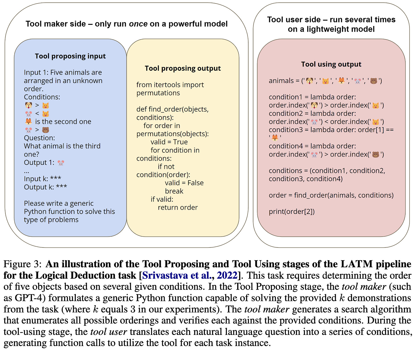
Why restrict your text model to calling existing APIs when you could have it write and execute its own Python code as needed? Or more precisely, why not have a big, powerful model write Python APIs once for your lightweight model to reuse many times?

You can kind of think of this as just having GPT-4 write Python functions for you and then using these functions in your smaller “tool user” model.

Except that they also have a Dispatcher model that determines whether a newly-received task can be addressed by existing tools and automatically invokes the tool maker (GPT-4) if not.

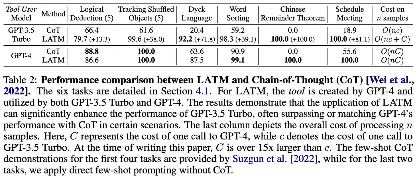
For tasks that can be solved with short Python functions, this approach can work super well.

This is really interesting but also seems like one of the most dangerous possible ways to use AI. Like, generating and executing untrusted code based on untrusted test-time inputs using a third-party API is about as insecure a piece of software as you could get. And having a model generate + execute code at runtime with no human oversight is pretty much the perfect setup for busting out of a sandbox and otherwise engaging in worst-case behavior.

So it’s cool research but I really hope patterns like this don’t become common in practice.

---

Scaling Spherical CNNs

Spherical CNNs are equivariant with respect to 3d rotations, making them a natural fit for problems in which objects can be in any orientation. This paper got spherical CNNs to work at a larger scale than previously achieved.

The core of the method is using spherical Fourier transforms, like in previous work.

But they add a number of optimizations. E.g., you can batchnorm in the frequency domain by just zeroing out the DC component and then dividing channels by their average squared entry.

These improvements together let them rival or surpass graph neural networks when making predictions about molecules. They also do really well at weather prediction.

They do take way more training compute than their baselines, but I’ll still call this evidence for the potential of CNNs with stronger [co,in]variances.

---

Error Feedback Can Accurately Compress Preconditioners

Some second-order optimizers use a history of gradients to estimate inverse Hessians or other preconditioning matrices.

This work proposes to compress these gradient histories using sparsity or factorization. They also add the running compression error to the next gradient to reduce compression noise.

When holding step count constant, this method can reach higher accuracy than SGD on various tasks.

It does take more memory and training time though.

In other news, they have a great summary of M-FAC. I hadn’t read about it before and feel like I mostly understand it after 3 paragraphs.

---

FasterViT: Fast Vision Transformers with Hierarchical Attention

It’s yet-another-ViT-variant *but* they have a speed vs accuracy plot on ImageNet that looks like this:

Which is even more thorough than the one from the recent EfficientViT paper, though the two seem to be operating in disjoint accuracy regimes:

The main idea in this paper is to use a certain form of hierarchical attention that lets every pixel depend on every other pixel without doing full quadratic attention.

The overall architecture looks pretty normal for a vision transformer, with a bunch of convs and downsampling early on and then attentions near the end.

One interesting facet is that the early layers of the network induce brightness-invariance (at least on average across a batch) thanks to the first batchnorm being preceded only by homogeneous functions. This is normal for a CNN but not what you normally see in a transformer.

It seems like their hierarchical self-attention does beat some alternatives when holding everything else constant. This is one of the few times I’ve seen a controlled comparison of attention variants with a clear winner (that wasn’t vanilla attention).

This attention variant also seems to be a relative maximum in the design space, in the sense that messing with pieces of it makes the model worse.

There are so many subquadratic attention variants that you can’t compare to them all, but this one does seem unusually promising—both simple enough to understand and better than alternatives even when controlling for throughput. I would actually try this if I were designing a vision transformer.

---

TASRA: a Taxonomy and Analysis of Societal-Scale Risks from AI

An AI risk paper from Critch + Russel, who IMHO are unusually credible sources. First, they note that “societal-scale” can mean either individual harm that’s widespread enough or harm to society as a system—think democracy, supply chains, or financial systems.

Given this framing, they construct a tree of possible scenarios and describe how each can go wrong.

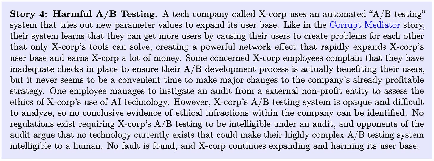
One aspect of that stands out is that they try to make their discussions concrete through hypothetical stories.

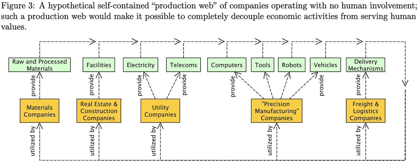
They devote a lot of space to how full automation can put humans in a bad spot, even if we don’t end up with large-scale poverty or unrest. Basically, if half your production is a bunch of AIs doing their own thing just trying to maximize output, they could “boil the frog” by being too painful to shut down at any given time but gradually getting more and more misaligned with our interests; e.g., they could ruin all the clean water, trash all the arable land, etc.

Definitely worth a read for anyone interested in risks from AI.

---

Fast Diffusion Model

Adding momentum to your diffusion steps makes sampling way better.

---

Learning the Positions in CountSketch

In a classical count sketch, we use a random sparse matrix to embed our data vectors in a low-dimensional space. Recent work has suggested optimizing the values of the nonzeros in this matrix based on a training set. This paper takes it a step further and lets you learn where the nonzeros go. They first choose the positions of the nonzeros and then optimize their values via gradient descent.

Their method trains fast, runs fast at test time, and yields lower error for a given matrix shape + sparsity count than alternatives. They also have strong theoretical guarantees.

As much as I love sketching algorithms and think they’re one of the most elegant corners of computer science, I have to admit that this paper reinforces my view that you should almost always use a directly-optimized alternative in practice.

---

Benchmarking Neural Network Training Algorithms

They release AlgoPerf, a time-to-result benchmark spanning a variety of workloads. They also discuss the many nuances of comparing across different algorithms and report some baseline results for different tasks. NadamW is surprisingly good when you don’t have Distributed Shampoo handy.

---

Unprocessing Seven Years of Algorithmic Fairness

Twenty different methods for improving the fairness vs accuracy tradeoff don’t beat a simple baseline when evaluated under controlled conditions.

---

INT2.1: Towards Fine-Tunable Quantized Large Language Models with Error Correction through Low-Rank Adaptation

They quantize LLaMA models using GPTQ and then finetune them with LoRA to match the output distributions of the original model. The LoRA weights aren’t quantized and don’t get fused in at the end, so the final model has a little bit of time and space overhead compared to pure int2.

There’s a significant quality drop at 3 bits and a huge one at 2 bits, which is interesting data. Looks like low-rank distillation can recover from 4-bit quantization but no lower.

---

Fast Training of Diffusion Models with Masked Transformers

Let’s say you’re training a vision transformer as your diffusion model. Normally you’d just noise up all the image patches and train the model to denoise them. They propose to instead split the patches into two sets at random and give each set a different objective:

• One set of patches gets noised normally and you train the model to denoise them

• The other patches get masked and you train the model to reconstruct them.

Because you can skip most of the computation for the masked patches, this variant can save a lot of compute.

It also seems to preserve image quality, at least to the extent that we know how to measure that.

---

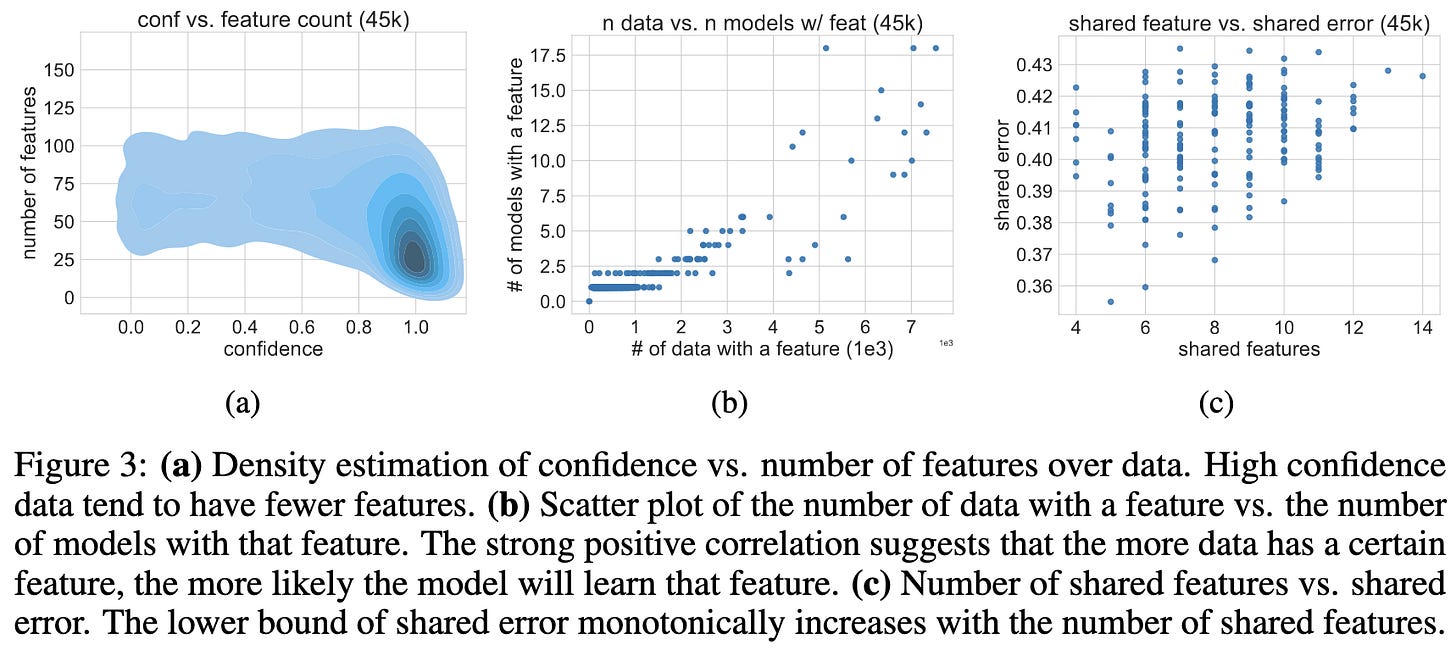
On the Joint Interaction of Models, Data, and Features

For image classifiers, the last-layer representations have concentrated principal components.

More surprisingly, classification accuracy on a given sample is correlated with the extent to which a few components dominate. Plus, more frequently-occurring components are more likely to be learned in independent training runs.

Basically, it seems that easier inputs get sparser representations. Though “sparse” doesn’t mean exactly zero here—just that a few components dominate.

This is consistent with previous work suggesting that model compression disproportionately wrecks accuracy on underrepresented examples.

---

Transformers learn through gradual rank increase

Consider the elementwise differences between the initial and current weights in a neural net. At least for the self-attention layers, this paper finds that these difference matrices gradually increase in rank over the course of training.

Interestingly, this is vaguely consistent with our above paper arguing that easy samples have lower-rank representations. I could imagine it being the case that models learn the easy samples early on, and gradually add more expressivity to capture the long tail. Also consistent with the quantization model of neural scaling, which argues that a) LLMs gradually gain discrete quanta of ability, and b) the quanta have a power law distribution of how often they come up.

---

1. If this paper’s scaling coefficents were worse, I would just conclude that the Chinchilla hand-tuned hparams worked better. But the fact that they’re nearly identical suggests that these coefficients are some sort of limit or attractor. Especially since the authors of this paper used a totally different LLM stack, which you’d expect to yield different results by default.

2. Note that this wouldn’t imply no improvement is possible for a given task. You could still train on better data, speed up your training stack, gain constant factor improvements in statistical efficiency, design better prompts, etc. You just couldn’t get better scaling with respect to dataset and model size.

Personally, my conjecture is that a) we can do better than the Chinchilla scaling coefficients, but b) probably not without significant methodological changes.

But I am really confident that we won’t get error rates to go down faster than O(1/sqrt(num_samples)) since I’m not aware of anything in all of statistics that does that.