2023-6-25 arXiv roundup: Learning from textbooks, Eliminating transformer outliers, Zero++
This newsletter brought to you by MosaicML.
Textbooks Are All You Need
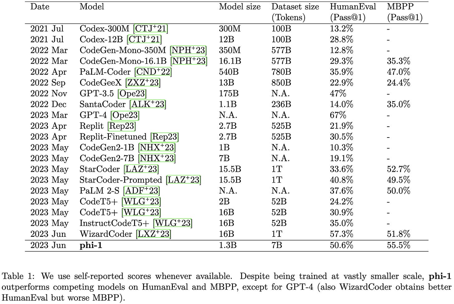
They got near-SotA code generation with a tiny 1.3B param model by curating an awesome training corpus.
This turns out to be possible because most code datasets are terrible. More precisely, they’re not self-contained; they lack meaningful comments, they’re mostly configuration or boilerplate; and they lack broad coverage.
To avoid these pitfalls, the authors construct a high quality code dataset of 6B tokens filtered from The Stack and StackOverflow and 1B tokens generated by GPT-3.5, with the latter designed to also include helpful descriptions.
They also construct the CodeExercises dataset, consisting of 180M tokens of Python coding exercises + solutions.
Pretraining on their CodeTextbook dataset and finetuning on CodeExercises works super well.
This is even more evidence for quality over quantity in training data.
It also makes me wonder about the superficial alignment hypothesis—maybe it just seemed to hold because the finetuning sets (e.g., LIMA) were super high quality? Experiments across different models holding the finetuning data constant seem like evidence against that though.
ZeRO++: Extremely Efficient Collective Communication for Giant Model Training
The DeepSpeed team improved on their ZeRO variants for distributed training (if you’re not familiar with it, my PyTorch FSDP writeup has an approximate explanation). There are three main optimizations here.
First, they have optimized CUDA kernels to convert f16 weights to int8 during the allgather, and then convert them back before using them.
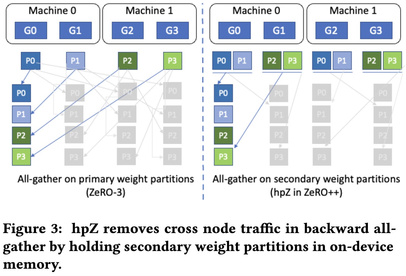
Second, they cache a full copy of the weights in each node, sharded across the 8 GPUs. This takes more memory but you can hit this cache for every forward and backward allgather except the first forward allgather after an optimizer step.
I find it kind of surprising that they treat this as a cache, rather than just doing hybrid sharding; I guess this way expands the regime where you avoid hitting RAM limits since your grads and opt states remain sharded across the whole cluster.
Their third optimization is rewriting their reduce-scatter ops to communicate in quantized int4 but upcast to f16 before applying the reduction op.
This is way subtler than it sounds because, with a regular ring all-reduce, you end up quantizing and dequantizing a number of times equal to the number of devices. To avoid this, they implement their all-gather as a two-level all-to-all, first communicating intra-node and then across nodes.
This doubles the number of scalars transmitted since it communicates a full set of gradients both intra-node and inter-node, but a) the total number of bytes transmitted stays the same thanks to the quantization, and b) the inter-node communication is cut in half, and that’s the bottleneck.
To get the most value out of these primitives, they track the execution order of layers and interleave the compute, intra-node communication, and inter-node communication.
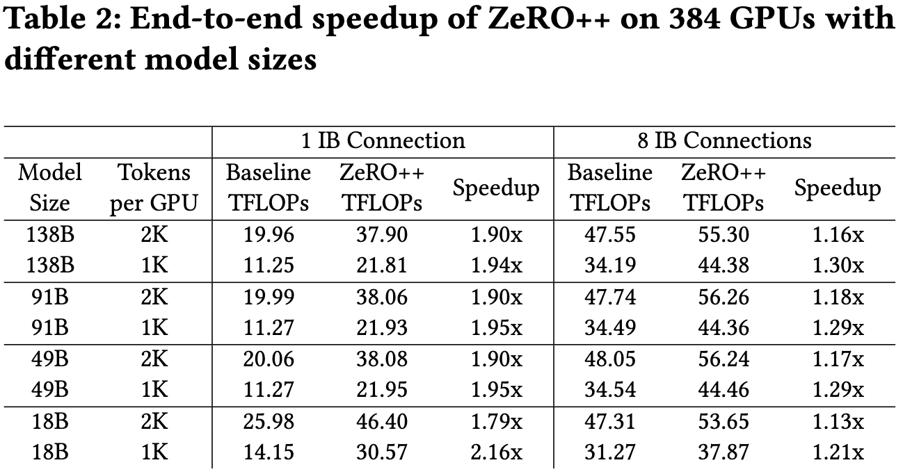
These optimizations together yield significant utilization lifts for various cluster and batch sizes. Results below are for 24 nodes of 8xV100s with 1 to 8 100gbps InfiniBand NICs.
As you’d hope, the individual optimizations are helpful in the relevant circumstances.
There also don’t seem to be appreciable convergence changes from the quantized communication. This surprised me since int4 quantization usually has an accuracy cost even for inference.
Solid systems work as always from the DeepSpeed team. I’m especially eager to try their quantized communication primitives.
Training Transformers with 4-bit Integers
So part of this is a clever extension of existing ideas, and part of this made me think “oh my gosh, you absolute madmen.” In a good way.
The first idea here is to precondition your weight and activation matrices before quantizing them by multiplying with an orthonormal, block-diagonal matrix. This is pretty typical for numeric data compression, but I’ve never seen it in a deep learning paper before.
The goal of this preconditioning is to equalize the variances of different features, spreading outliers across the whole vector. And it does a great job of that.
The particular matrices they use as their block-diagonal tiles are Hadamard matrices, which have nice properties like letting you multiply with them in N^2*log(N) time instead of N^3. Interestingly, people have previously used Hadamard transforms to improve differential privacy guarantees; so that’s two subfields in which they’ve been helpful for reducing outliers.
That’s how they change the forward pass. In the backward pass, they do something crazier. The observation they’re trying to exploit is that the gradient matrices often have entire rows that are tiny or even zero.
They capitalize on this by sampling rows of the gradients and activations based on leverage scores, which choose larger rows more often.
Dynamic structured sparsity is already aggressive. But what really adds gas to the fire is their choice to quantize the relevant matrices to 8 bits and treat the high 4 bits and low 4 bits as separate matrices.
The idea is that:
Two int4 matmuls is almost as fast as one int8 matmul
But the high bits will only be nonzero for large-ish values, which are uncommon. So when downsampling, you can skip more rows in the high bits’ matmul.
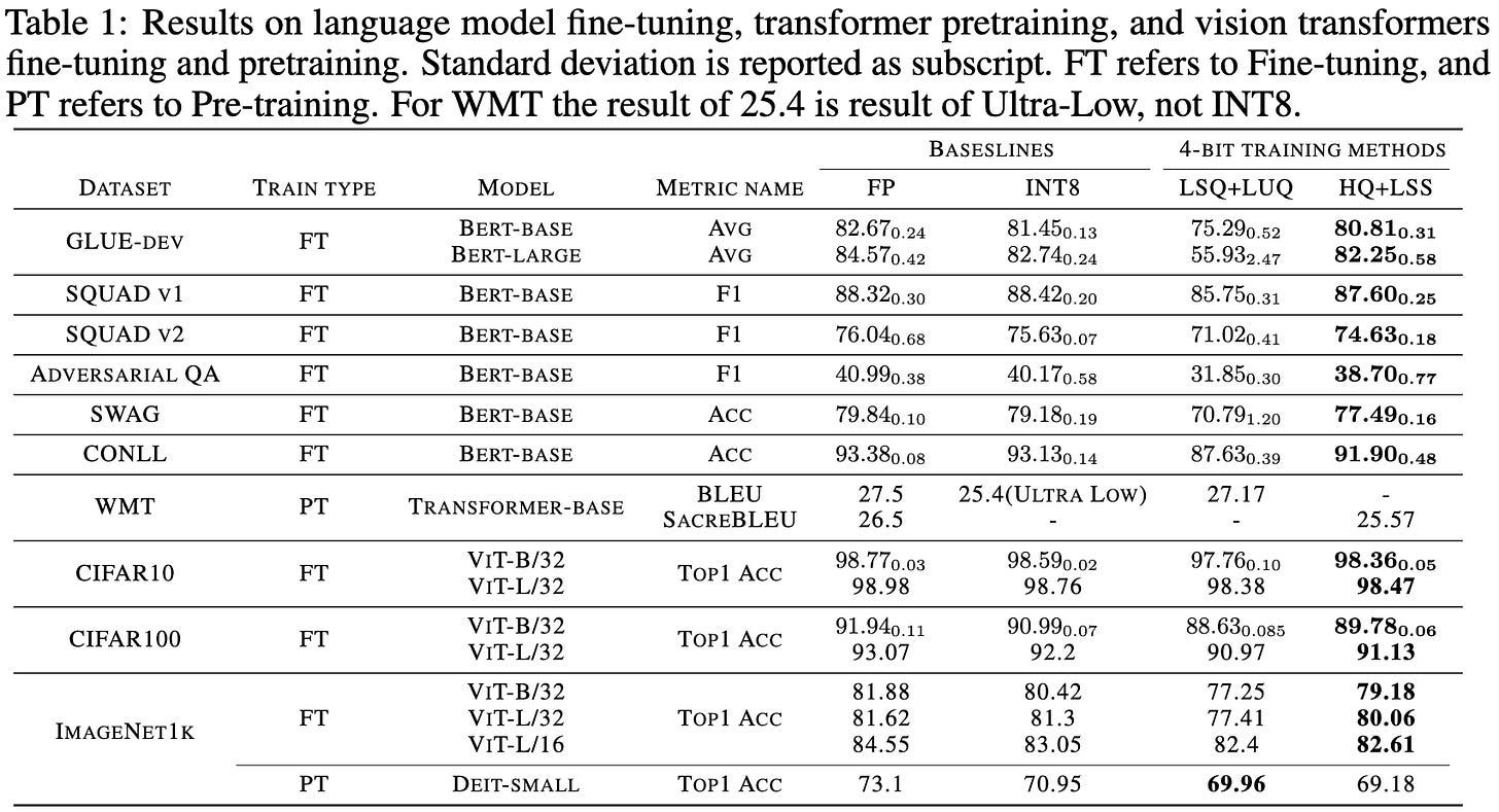
They don’t quite get to the accuracy of int8 training and are a few percent behind f16 training, but they do beat a sensible 4-bit alternative.
They also wrote some serious CUDA kernels using CUTLASS and managed to get their quantized ops to run fast. I’m not sure how the Hadamard quantization (green bars) is more TOPS than the int4 matmuls though—maybe because the structured matrices let them exceed the nominal peak?
So it’s definitely not a drop-in replacement for [b]f16 training, but I have mad respect for not only trying something this ambitious, but building the kernels to get real throughput numbers.
No Wrong Turns: The Simple Geometry Of Neural Networks Optimization Paths
With a decent batch size, your gradients almost always point in the same direction as the difference between your current and final weights. “Point in the same direction” is defined as cosine similarity > 0.
This result isn’t trivial; if you optimize other functions known to be non-convex, you don’t get this property. This suggests that neural net loss landscapes have some non-obvious structure.
They also do some math to derive the (locally) optimal learning rate at a given step; this optimal rate often warms up quickly, then decays throughout training—consistent with common practices.
Filing this away in my mental “deep learning phenomena that need to be explained” folder. Which is a super valuable folder for guiding us towards a physics of deep learning.
Deep Fusion: Efficient Network Training via Pre-trained Initializations
They do the thing where you initialize a wider model from a narrower model by using the narrow weights as the upper left of each widened matrix and zeroing the rest—except they initialize from two half-width models instead of just one smaller one.
This can improve your time to accuracy for T5 models compared to a random initialization.
Almost equivalently, you can improve time to accuracy. There are some subtleties around handling the layernorms—do you normalize the two halves of the features separately, or together? It turns out you should layernorm the halves separately (“fusion-prop” in the table).
It seems to work better to fuse two different models than two copies of the same model, at least for T5-medium on GLUE. Makes sense that redundant weights wouldn’t be as good as diverse ones.
Mostly I feel like initializing wide models with narrow models just seems like a free win given good software support. E.g., maybe we should initialize MPT-30B using MPT-7B?
Understanding Parameter Sharing in Transformers
Parameter sharing across layers is super interesting from a scaling perspective because it increases your FLOPs without increasing your parameter count. So what happens when you share params in various ways?
First, we need to think about what the different ways of sharing parameters there are.
The easiest method is just repeating the same layer multiple times. This either decreases the param count or increases the depth, depending on whether you add new layers.
Two less obvious variants are “sharing in branches” and “sharing in matrices”, where you hold depth constant still share across layers, but also widen the layers to compensate for the sharing.
In terms of steps, they find that you might do better with parameter sharing.
But in terms of wall time, you don’t really do better than the baseline when using the same, optimized hparams.
So…kind of seems like you don’t want to scale up FLOPs and activations without parameters, at least for the transformers they use. This is consistent with MoE results suggesting that scaling up parameters without increasing FLOPs works really well.
Scaling MLPs: A Tale of Inductive Bias
What if we scale up MLPs instead of transformers?
For one thing, you want to spend your compute on more data and fewer parameters than in a transformer. This is consistent with the framing that MLPs have worse inductive bias / are less sample-efficient.
A corollary though is that you can make up for the lack of inductive bias in MLPs with more data + parameters. So transformers can be an efficiency win, but don’t have any magic that MLPs can’t match at greater cost.
These results make a lot of sense. they also seems like mild evidence against my conjecture last week that the Chinchilla scaling coefficients are some sort of attractor or statistical limit. They could be a limit since the MLP scaling is worse, but they’re probably not an attractor (at least outside of specific architectures and training practices).
Revealing the structure of language model capabilities
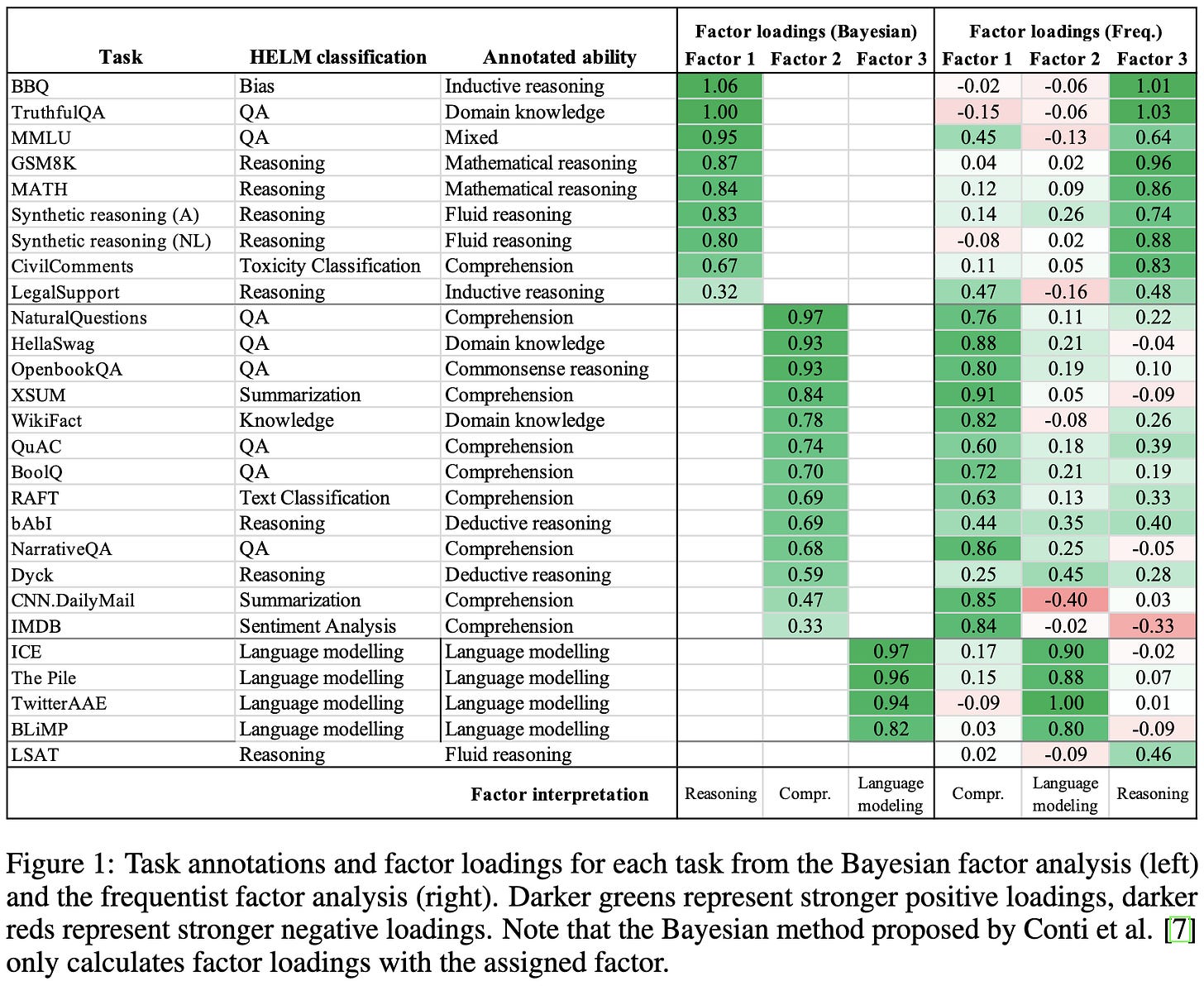
They ran a bunch of eval suites on a bunch of LLMs and analyzed the patterns in the results.
They found that you can explain 82% of the variance across different tasks by using three latent factors, which can be understood as “comprehension”, “language modeling”, and “reasoning”.
All three factors go up with model size, but language modeling (unsurprisingly) goes down with instruction tuning.
The presence of distinct groups of capabilities, as opposed to a single notion of intelligence, is consistent with FrugalGPT, LLM-Blender and other findings suggesting that different models have different strengths.
Any Deep ReLU Network is Shallow
Your deep ReLU network can be converted to an equivalent 3-layer ReLU network. Maybe not efficiently, but it can be done. This is cool because this isn’t an approximation theorem—it’s an equivalence, which is much stronger.
An Overview of Catastrophic AI Risks
A 50-page rundown of ways AI could go really wrong. A one-stop-shop for various arguments and scenarios you’ll encounter if you spend enough time on rationalist forums.
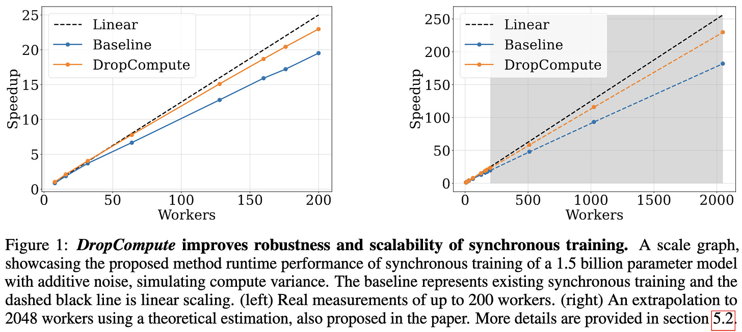
DropCompute: simple and more robust distributed synchronous training via compute variance reduction
A Habana paper that speeds up data-parallel training using a simple intervention. Namely, they have all the workers just stop computing gradients after a certain amount of time. Assuming the clocks are synchronized, this eliminates stragglers entirely, in exchange for earlier layers getting only partial gradients from some devices.
This works in the case that you’re doing gradient accumulation, so that all workers have some gradient for each parameter—it just might be missing the contribution of the last microbatch.
I was surprised to see just how much variation they observed in step time across workers—though I’m not sure about the hardware setup here (e.g., GPUs vs Gaudi).
This dropping of stragglers doesn’t seem to mess with model quality.
And it enables up to a ~5% speedup on Gaudi chips.
You’ll lose determinism, but otherwise this seems like a pretty straightforward win once you have enough stragglers and microbatches.
Graph Ladling: Shockingly Simple Parallel GNN Training without Intermediate Communication
I don’t read many GNN papers, but you had me at “shockingly simple”.
They sample/partition their graph, train a separate GNN on each graph, and then interpolate the GNN weights using model soups.
This apparently works really well:
Neural Priming for Sample-Efficient Adaptation
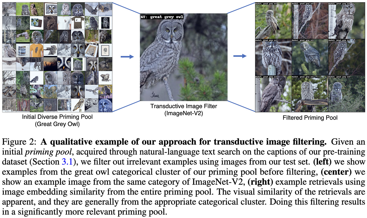
They retrieve training samples relevant to a given test input and use these samples to perturb the final classification layer of an otherwise-frozen CLIP model.
To improve the speed and quality of the retrieval, they choose a subset of the training set as the retrieval corpus. This subset is formed by filtering the training set based on whether their captions match test-time class labels and whether CLIP thinks the captions align with their images. When the whole test set is available at once, they further filter by taking the union of the 10 nearest neighbors of all test images.
Given the retrieved images for a given test input, they adapt the final linear classifier by biasing it towards a closed-form linear classifier that would classify the retrieved images correctly.
They tuned a lot of knobs here, but the accuracy lifts across a variety of different datasets are large and consistent.
The method works way better when you have more samples per class.
It doesn’t seem to matter how big your model is though.
The choice to condition on test samples by perturbing the last layer is both unusual and interesting; maybe we should be doing this whenever adding retrieval to a classifier? If we can get this to work a) outside of just CLIP models and b) with fast enough retrieval, this could be a promising way to lift test accuracy.
Quantizable Transformers: Removing Outliers by Helping Attention Heads Do Nothing
They argue that the following process is responsible for outliers in transformers:
The attention layer would “like” to output zeros so that the residual stream doesn’t get updated for some features and/or some tokens. E.g., you don’t need to do much updating for the [SEP] token.
To approximate a no-op, an attention head tries to allocate all its attention to near-zero inputs like padding or uniform background patches.
But to allocate as much attention as possible to certain tokens, the softmax needs the largest inputs it can get. And since there are layernorms all over the place, you need some huge activations for certain attention entries to dominate. I.e., you need outliers.
Worse, since the softmax only approaches being a categorical distribution, the model will always try to grow the weights, and the outliers get worse the longer you train (or until weight decay forces an equilibrium?).
To fix this behavior, they propose two changes to the model. First, they propose to gate each token in each attention module using a small, learned, gating network.
Second, they propose to clip the softmax by stretching its values outside of the interval (0, 1) and then clipping to (0, 1). This adds hparams but lets the attention express 0 and 1 exactly and without large logits.
Fortunately, the exact clipping hparams don’t seem to matter much as long as they’re slightly outside (0, 1). Extending below 0 seems especially important.
These proposed changes each improve accuracy, both in fp16 and in int8 when doing post-training quantization.
This is awesome. In one paper we have thorough probing of what’s really happening in an important phenomenon, a unifying + testable hypothesis, and interventions based on that hypothesis that work well in practice. This is a quantization paper I’m probably going to come back to a lot.


