2023-4-23 arXiv roundup: Adam instability, better hypernetworks, More Branch-Train-Merge
This newsletter made possible by MosaicML.
Also: is anyone looking for a podcast guest? I may or may not have a podcast in the works and want to get experience being on the guest side of the table. Feel free to just reply to this email if you know anyone who’d be interested in having me come ramble er, uh, share brilliant insights.
Non-Proportional Parametrizations for Stable Hypernetwork Learning
They made hypernetworks work better by identifying and fixing one of their main pathologies.
For those unfamiliar, hypernetworks are neural nets whose output is another neural net; this lets you do stuff like feed in a desired image resolution and get out a model specialized for that resolution with no extra training.
The biggest issue they find is that the output tends to be proportional to the input. This provably happens if all your nonlinearities are piecewise linear functions.
We’ve previously seen this observation used to make networks invariant to input scaling through explicit normalization. In this case, they skip the normalization and use a more general (and probably faster) approach. First, they have the network produce changes to the parameter values from a default initialization, rather than the parameter values themselves.
Second, they encode each input scalar using a sine and cosine function. Interestingly, this also works really well for stuff like implicit neural representations of point clouds.
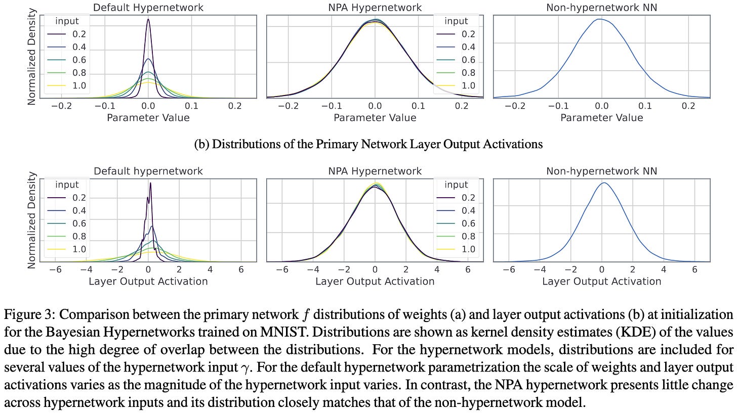
With these two changes, they get the output variance to be consistent across input values. This leads to a number of desirable properties. For one, they get much stabler gradient norms.
More importantly, the networks produced by their modified hypernetwork tend to work better for downstream tasks.
They also find that their fixes work better than (even) simpler solutions like just sticking normalization layers in the hypernet.
These improvements seem to hold across a variety of different architectures. Although note that all the reported results are just with fully-connected networks.
Nice to see a well-executed paper making substantive improvements to hypernets. They’re a really interesting alternative to using a pretrained model directly—they could in principle allow you to get a smaller task-specific model, which could lower both finetuning and inference costs.
Research without Re-search: Maximal Update Parametrization Yields Accurate Loss Prediction across Scales
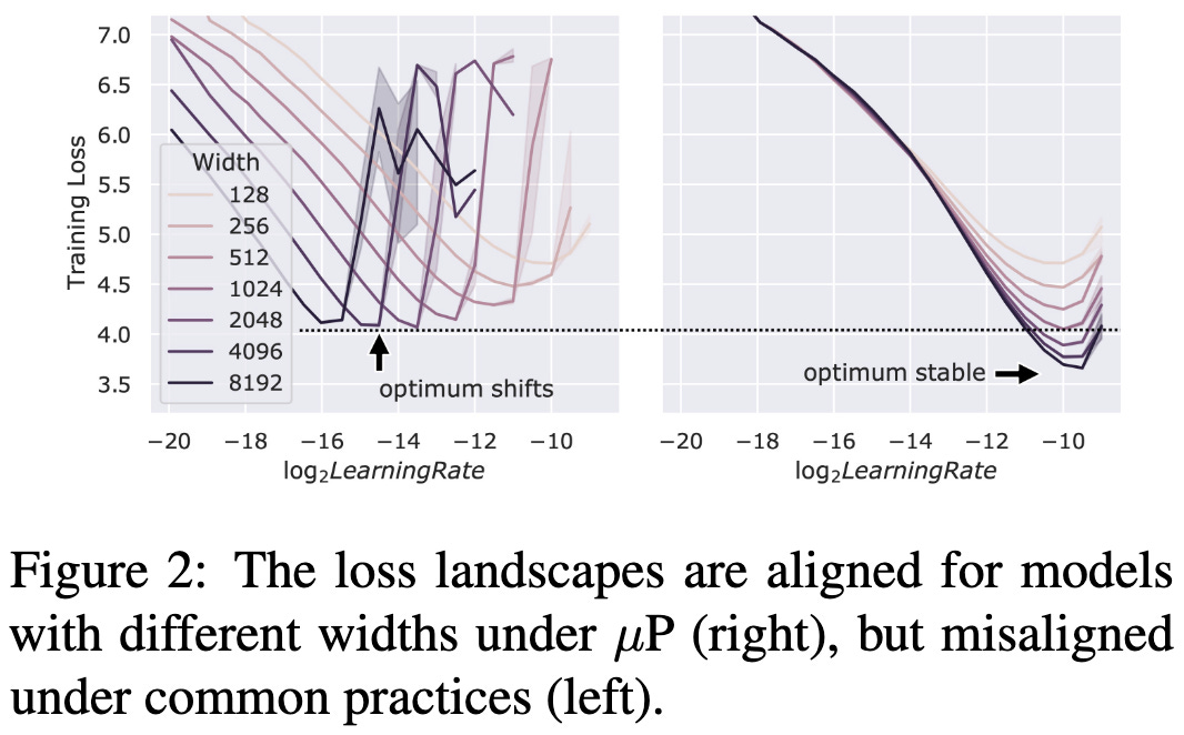
They reproduced μTransfer and found that it gives you power law scaling without having to change the hyperparameters at different model sizes.
You do still have to choose decent hparams though for everything to scale well; it’s just that you can use those same hparams at all scales.
It’s not trivial to obtain this property—you don’t get the same scaling behavior without muParameterization.
Between this and CerebrasGPT, it looks like muTransfer really works—at least for text models. Also, as this paper highlights, we might be able to use this reliable scaling to compare small-scale results directly to large-scale ones (assuming the extrapolation is reliable enough).
Calibrated Chaos: Variance Between Runs of Neural Network Training is Harmless and Inevitable
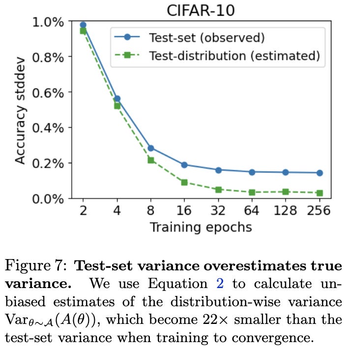
They have a few findings about test set variance across thousands of CIFAR-10 training runs. First, the variance tends to decrease the longer you train.
More interestingly, training for longer removes correlations between the accuracy on different subsets of the test set. I.e., getting “lucky” on half the data predicts also getting “lucky” on the other half early on, but not after enough training. I’m reading this as “random variations make some models actually better early in training, but not later in training.”
By the end of training (but not at the start), getting each example right is an independent event that happens with some example-specific probability.
Relatedly, the true variance of the trained model on the test distribution is probably much lower than the empirical variance on a finite test set.
The above CIFAR-10 observations also seem to hold for ImageNet-1k. The observations no longer hold when there’s distribution shift between the train and test sets (e.g., for ImageNet-Sketch).
There are a bunch of other results in this paper as well, but I found it both interesting and encouraging that example-wise independence seems to hold.
Tool Learning with Foundation Models
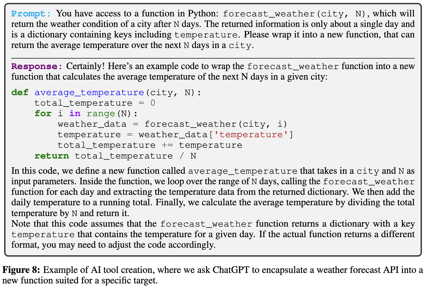
A 73-page survey of tool use in big, pretrained models.
They also evaluate a variety of different tools one can use with text-davinci-003 and ChatGPT.
Synthetic Data from Diffusion Models Improves ImageNet Classification
You can do pretty well on ImageNet-1k by just replacing the real training data with AI-generated images. If you augment the real training data with AI-generated images, you get a big accuracy lift.
Though of course, the generated images have to be really good and you might need to mess with the generator hparams.
In fact, to make these accuracy gains possible, they have a special finetuning pipeline for Imagen that achieves a new state-of-the-art for FID and Inception Score on ImageNet.
Their results suggest that having this high image generation quality really does translate to better classification accuracy.
Also, these accuracy lifts hold across a variety of different models and resolutions.
How many synthetic images should we add to our training data? They find that you get accuracy improvement initially, but eventually it gets worse than the baseline. Makes sense from a bias-variance perspective—you trade a little bias for a lot of variance reduction initially, but later the bias becomes too large.
Pretty cool. Another example of using machine learning to generate training data for machine learning.
Visual Instruction Tuning
Let’s say you want a chatbot that can take in both text and images.
A big problem is that there isn’t much training data for multimodal chat. So what they do is use a pretrained object detector and a pretrained text model (in this case, GPT-4) to generate a conversation about a captioned image. The prompt to the text model is the set of image captions along with object classes and bounding boxes (but not the image). They design some prompts to elicit conversational responses about these inputs.
They finetune LLaMA on this expanded dataset. They also turn the image into a set of embeddings using an image encoder and feed these embeddings into the model along with the text token embeddings.
The resulting model can be pretty impressive, talking about the content of images even without access to an object detector.
Remarkable how fast we went from automatically generating instruction tuning data for just text to text + images.
Also, shoutout to Jim Fan’s twitter thread for helping me understand this paper.
Amortized Learning of Dynamic Feature Scaling for Image Segmentation
So you know how we always downsample by a factor of 2 throughout our CNNs? You can probably do better than that if you’re willing to treat the downsampling factor as an hparam, but boy would that be annoying.
This paper proposes to give you the speed vs accuracy lift of tuning the downsampling factor but without the pain of hparam tuning. The way they do this is via hypernetworks. Concretely, they train one hypernetwork to generate networks with different downsampling factors. This allows you to choose the speed/accuracy you want with just a single training run.
The method is pretty simple. They just have an MLP as the hypernetwork and sample a scale factor at each training step. Because the created model is just convolutional and elementwise layers, they can use the same number of parameters for all scale factors.
Empirically, this actually works better than just training a model directly using each scale factor. Since the inference-time parameter- and FLOP-counts are the same in both cases, this might be an interesting case of training compute on its own improving results?
You might wonder: since the same weights can run with any scale factor, is the hypernetwork just spitting out one really good network every time? The answer is no; if you take the weights for one scale factor and use them with a different scale factor, it works worse as the gap in scale factors increases. Although they’re still more robust to the scale factor than the weights from a regular U-Net.
Between hypernets and cyclic learning rates, it looks like we might be able to construct time vs accuracy Pareto frontiers much more quickly in the near future.
A Theory on Adam Instability in Large-Scale Machine Learning
If you’ve ever trained a large language model, you’ve probably had to deal with loss spikes. This paper asks: what’s up with those?
Before we talk about what’s happening, we first need to recall the terms in the Adam update formula:
We’ll also be discussing r_t, the ratio of m_t to sqrt(v_t). This is what the update approaches as ε → 0.
So here’s what they suggest is happening (see page 11 for a more detailed discussion):
Initially, training is going great. r_t is way above epsilon and we’re getting nice distributions of gradients. In particular, our update is large enough that the gradients we see across different time steps are centered around 0 and nearly uncorrelated.
Over time, the gradients for some subset of the parameters (often the early layers) start to vanish. More precisely, m_t, sqrt(v_t) ≪ ε. This makes the update for these parameters go to zero.
Since our parameters aren’t changing much and we often have a large enough batch to average out a lot of the inter-batch gradient noise, we end up getting basically the same gradient for our slow-moving parameters at every time step.
This causes r_t → ±1 (depending on the sign of a given parameter’s gradient, since v_t is always positive). And therefore u_t (the update) becomes bimodal as well—just squashed towards 0 because of the ε in the denominator.
At this point, learning is slowed but not diverging. The divergence happens when some parameter(s) somewhere finally get a gradient much larger than ε. The numerator makes m_t go way up, but the denominator (dominated by ε, not sqrt(v_t)) stays nearly the same. This leads to a huge update to some parameters.
This update is often large enough to knock the network into a higher-loss part of the landscape, triggering a chain reaction in which more parameters get huge gradients relative to their denominators.
But, with the parameters moving around again, the m_t values in the numerator start averaging to 0 and the denominators start getting bigger. This stabilizes everything and completes the cycle.
I’m not clear on why the bimodality matters, but this process makes sense overall. And increases my conviction that standard practices for neural net training are madness from a numerics and stability perspective.
PopulAtion Parameter Averaging (PAPA)
They train a bunch of different models and average them together during training. This improves accuracy compared to just training one model, and doesn’t have the inference cost of using the separate models in an ensemble.
There are three variants here. The first two just average the weights from different models periodically.
The two variants are distinguished by whether you average across all of the models or random subsets of m models.
The third variant moves each model’s weights towards the average instead of setting them equal to the average.
These algorithms are similar to Model Soups, but with the averaging happening throughout training instead of just at the end.
Using their method’s third variant (shrinking towards the average) and then averaging the models at the end seems to work the best for ResNet-50 on ImageNet. It’s not as good as ensembling the models, but it’s better using any of the individual models.
Their variants also seem to do better than training a single model for longer; by “longer,” I mean the duration is scaled up by the number of models in the set. This at least works when using 10 models on CIFAR-100.
This paper is another interesting datapoint regarding linear mode connectivity and model averaging.
Scaling Expert Language Models with Unsupervised Domain Discovery
A follow-up to branch-train-merge in which they discover clusters in the data rather than assume explicit “domains” annotated ahead of time. The clustering is k-means on TF-IDF features with exact cluster balance enforced during the optimization (but not at inference time).
If you don’t remember branch-train-merge, they just start off with one “seed” model, make k copies of it, train the copies on disjoint subsets of the data, and then make predictions using a weighted subset of the copies. The idea is that each copy becomes an “expert” in one part of the input space.
To make predictions, they route each sequence to an appropriate subset of the models based on their learned clusters, then average these models’ predictions.
The output of each expert is weighted based on the distance between the input sequence and the cluster centroid. Only a subset of the experts receive a given input.
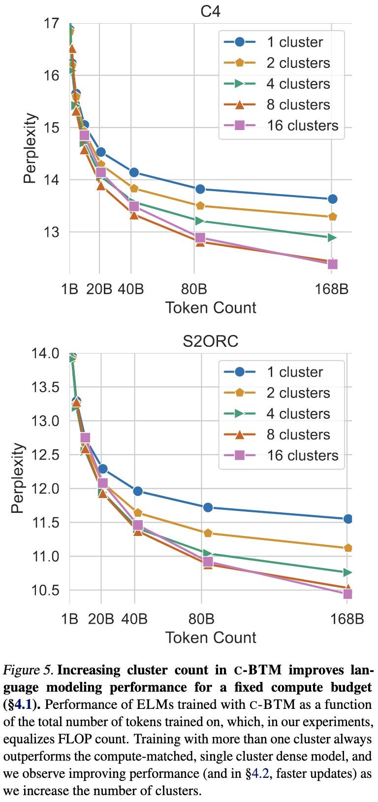
The main result is that, for a given training budget, this method tends to do better than just continuing to train the seed model.
In terms of perplexity, you almost always do better using more clusters.
This result holds all the way up to 6.7B param models, although they only trained for 21B tokens at this scale.
You can get some massive accuracy lifts on downstream tasks if you’re willing do a lot more work during inference—though there isn’t a predictable, monotonic relationship here. The extra work is from using more than one model.
Their approach does better than a more typical mixture of experts construction.
In terms of ablations, they find that using meaningful clusters—rather than random ones—is important.
It’s also important that the clusters be balanced during the cluster learning phase.
You pay a big space cost with this approach, but a method for turning space into accuracy could be really valuable.
This is also interesting data regarding what’s happening with regular MoE—it seems to go against findings that random routing can work just as well as trying to make experts specialize. Maybe the reconciliation is that routing in normal MoE models is so terrible that the specialization is dominated by the routing-induced variance (perhaps due to representation collapse)?


